Week 9 - FVM Literature Review

Week 9 - FVM Literature Review

Aim : Review of the Finite Volume Method

Since, the Finite Difference Method is simple to use for discretization of grids, it cannot be put into practice if the grid structure is not completely aligned along axes.

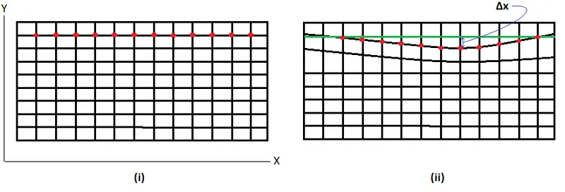
However, some interpolations can be made, to compensate the effect of shifted grids, but continuing the same approach with Finite Difference Method is not reliable. Such issue is not desirable if the meshed geometry of interest is 2D, and is not possible to implement such schemes if the geometry is 3D.

On the other side, in the Finite Volume Method, instead of defining the governing equations at the grid points as is done in F.D.M., the equations are written up for a volume, then the mathematical techniques are applied to help solve these equations for any type of grids, including non-uniform.

In F.V.M., the governing equations are represented in the conservative form, with application of Gauss's Divergence Theorem (linking surface and volume integral).

Consider the 1D Steady State Heat Conduction equation, where F.V.M. is applied,

`alpha(del^2T)/(delx^2) + S = 0`

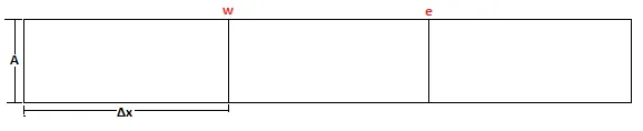
Applying for a volume cell,

`int [del/(delx)(alpha(delT)/(delx))]dV + intSdV = 0`

`int [del/(delx)(alpha(delT)/(delx))]Adx + intSdV = 0`

`[alphaA(delT)/(delx)] + SdV=0`, as its applied from cell face 'w' to 'e',

`alphaA(delT)/(delxe) - alphaA(delT)/(delxw) + SdV =0`

`alphaA((Te - Tp)/(Δx)) - alphaA((Tp - Tw)/(Δx)) + SdV =0`

From the above eq. the first two term represents heat fluxes, representing the temperatures numerically as "gradient schemes". Now as the flux terms are written for faces 'w' and 'e', in case if the thermal diffusivities are required to be estimated at both the faces, then prior to it, temperatures are needed to estimated first, as an "interpolation scheme".

The Gauss Divergence Theorem can be represented as;

`∯veca.n.vec(dA) = ∰nabla(veca)dV`

Here, `veca`= vector

`n` = normal vector

`vec(dA)` = elemantal area

`dV` = elemental volume

The General Scalar Transport Equation for a control volume is given as;

`del/(delt)∰(rhophi)dV + ∰nabla(rhophivecu)dV = ∰nabla(Γnablaphi)dV + ∰SdV`, `

Now applying the Gauss Divergence Theorem to the above Transport Equation, we have;

`del/(delt)∰(rhophi)dV + ∯(rhophivecu)dA = ∯(Γnablaphi)dA + ∰SdV`

The above equation represents summation of "rate of increase of `phi` inside control volume plus rate of `phi` fluxing out of control surfaces " is equal to "rate of increase of `phi` thru diffusion plus increase in `phi` due to source".

Here, the two terms are converted to the "control surfaces" from "control volume", if this is not done then the control volume can be represented via one cell centroid, on which everything will be dependent. There will not be any connections to the neighbour faces, and so the equations will get disconnected.

The Finite Difference Method, having non-conservative form of equations, does not involve integration on a particular control volume, so Gauss Divergence Theorem cannot be used, so the F.D.M. will not result in conservation on cell by cell(elemental) basis, whereas this is satisfied by the Finite Volume Method.

The final solution of a simulation will be same by the Finite Volume or by the Finite Difference Method, however the path to the solution is different. The goes thru the sequence of conservation equations for Finite Volume Method, whilst via Finite Difference Method, it may not go conserved.