Week 9- Unsteady moving zones Approach
Week 9- Unsteady Moving Zones Approach
The present problem is the continuation of previous problem specification, with a slight modification.
Here the case is ran as a time marching problem.
The mesh files are appended as a case in Fluent and cell zone conditions are defined as fluid for all.
Boundary Conditions:
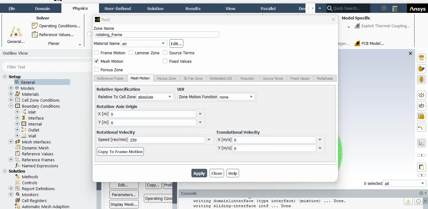
For the Boundary conditions, the Rotating frame, i.e. Zone 2 is kept in Mesh Motion instead of the Frame motion with input angular velocity of 300 rpm.
With regards to the boundary conditions, the respective zones, with 'Frame3_inner', 'domain1inerface' and both the rotating domains are given interface condition.
The airfoil wall is set to Moving will with motion respective to adjacent cell zone, i.e. Zone 2 (rotating_frame)
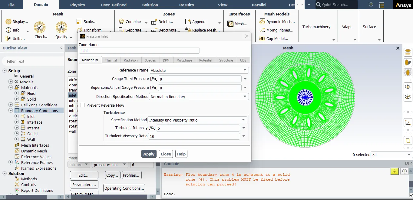
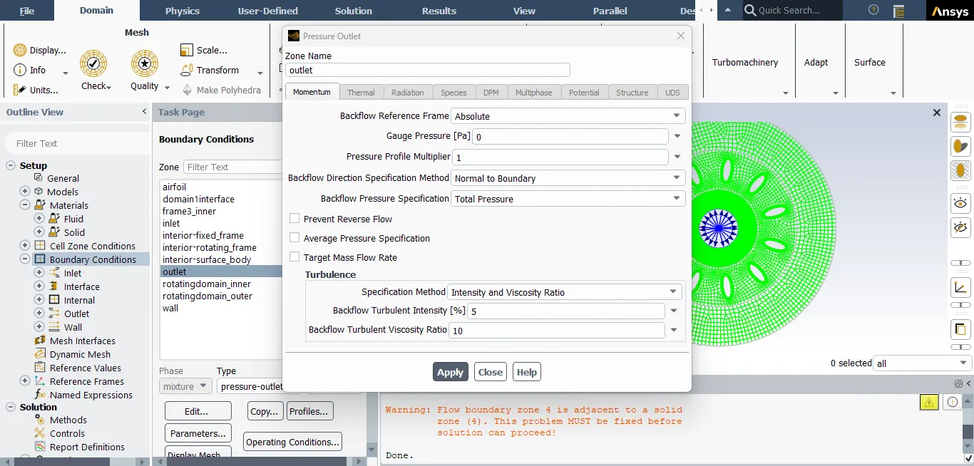
The Inlet and Outlet are provided with Pressure-Inlet and Pressure-Outlet conditions respectively, as there is no pressure difference.
The viscous model is set to k-epsilon Realizable, with enhanced wall treatment as it is the case for the rotating flow.
Mesh Interfaces:
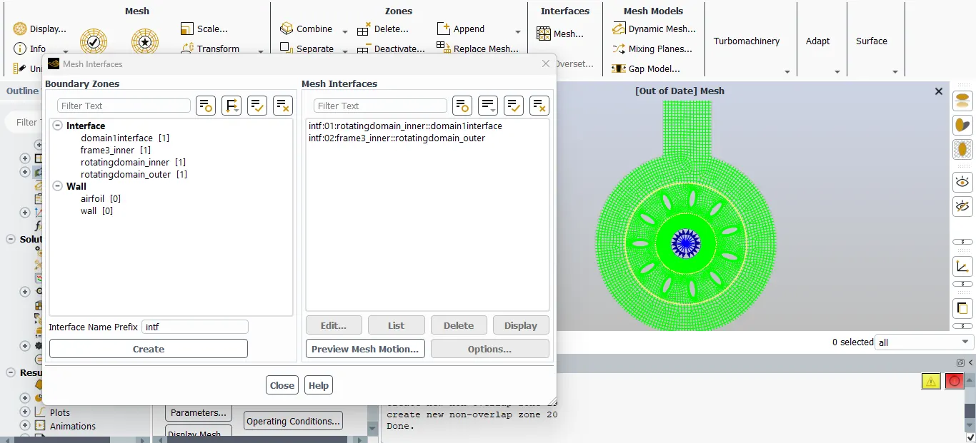
As the mesh for 'rotatingdomain_inner' and 'domain1interface' will overlap. an interface is set for both of them. The similar will be applicable for 'frame3_inner' and 'rotatingdomain_outer'.
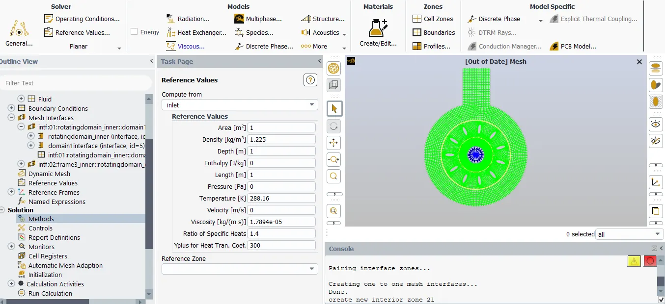
Reference Values:
The reference values are to be calculated from the inlet based on the input conditions provided.
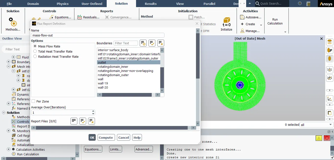
A definition of calculating the output mass flow rate is provided.
Solution Control and Method:
The Flow Courant number is kept to 10 as previous case. This variation in CFL number could be from 0 to infinity based on the suitable time-step size and total iterations to be performed per time-step to achieve the convergence.
The Pressure-Velocity scheme is set to 'Coupled', with Turbulent Kinetic energy and Specific Dissipation Rate set to Second order upwind.
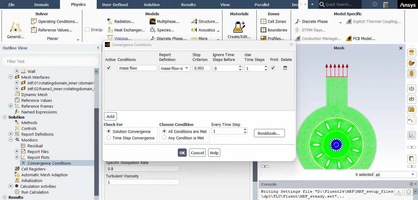
A Convergence criteria for the Output mass flow rate is defined as follows;
For calculating the Mass Flux, the flux scheme is set to 'Rhie-Chow Distance based'.
The initial values for the solution are guessed based on the Hybrid initialization.
Time Step and iterations:
The angular velocity is `N`=300 rpm, this can be equated as:
`omega = (2*pi)/T = (2*pi*N)/60`
`T = 60//N` = 0.2 seconds
Thus, to achieve this period within 1000 time steps, Time-Step size will be;
`Δ T = 0.2/1000 = 0.0002 s`
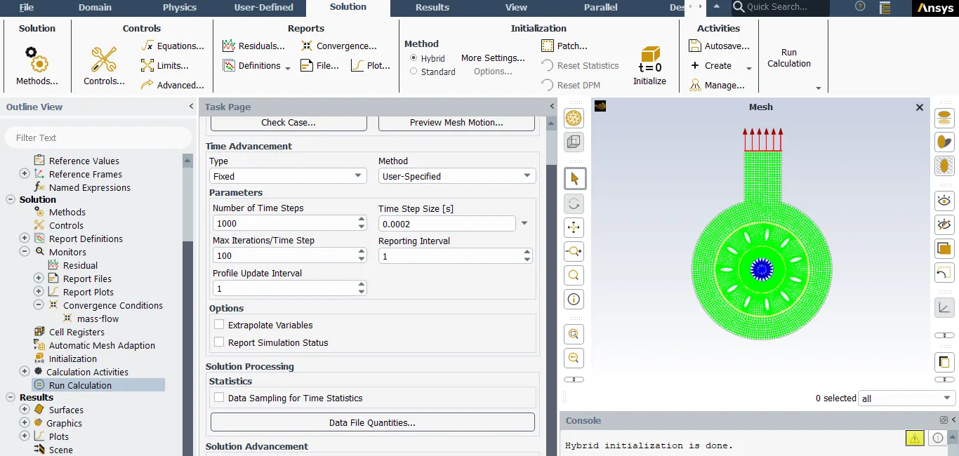
Since it is a Transient case, a time dependent solution file is created showing the variation in Velocity and Pressure.
Contours:
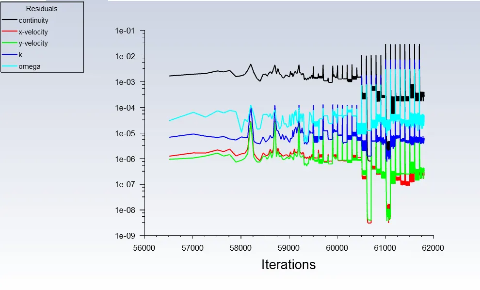
1. Totol Iterations
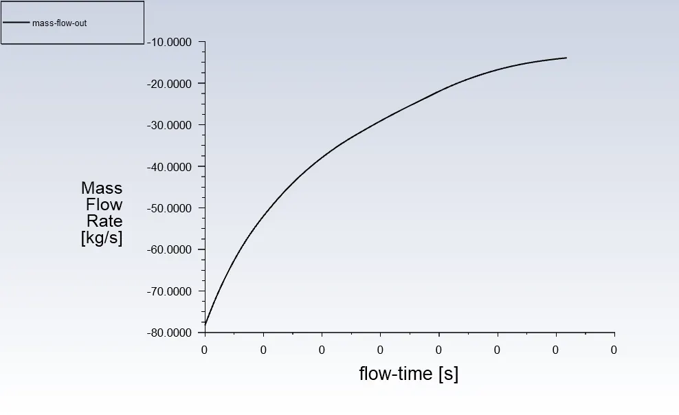
2. Outlet Mass Flow Rate variation for the Transient Case
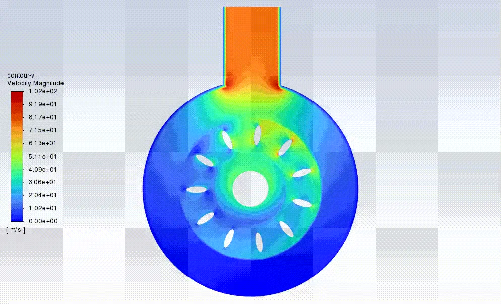
3. Contour of velocity
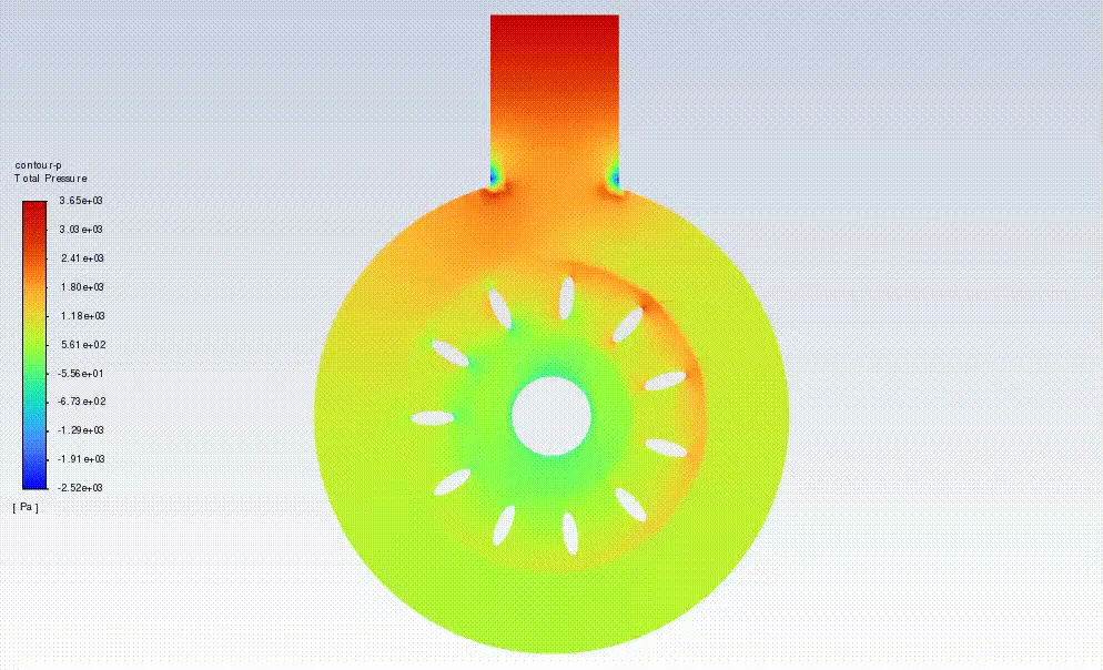
4. Contour of Total Pressure
Conclusion:
From the contours presented above, it is clear that the case has not yet reached the steady state yet. With time, there is variation in Total pressure and Velocity.
Furthermore, the current Mass Flow Rate for provided number of iterations is something about 15 kg/s, and the iterations are not yet converged, so the solution needs to be ran for more iterations to visualize the steady state reached.