Week 7 - Minor Project
Week 7 - Minor Project
Geometry Setup:
The project starts by importing the .DAT file of NACA0012 airfoil to ICEM CFD.
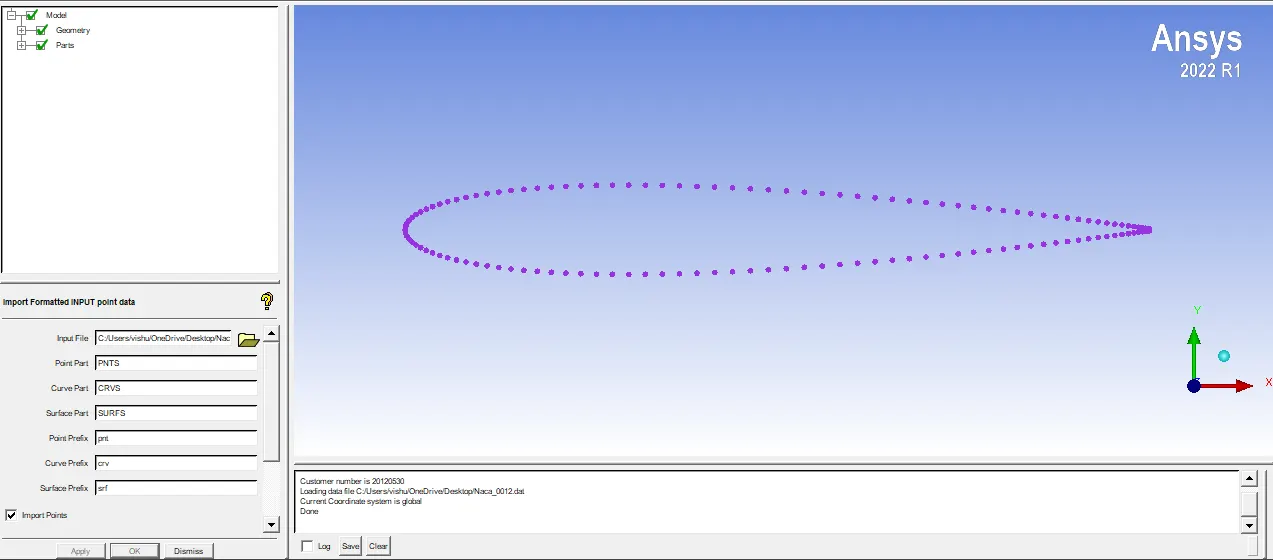
After that all the points are joined by forming a curve.
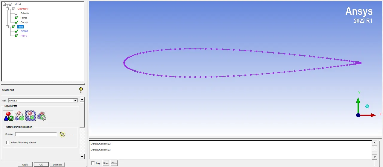
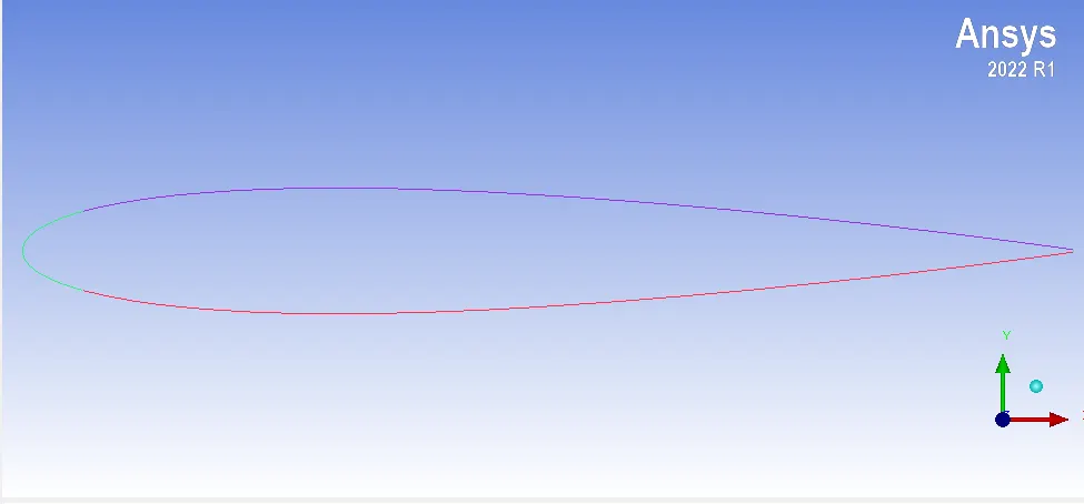
Secondly the parts are created for the air fold surfaces.
In the next stage the domain length is defined by creating the points around the airfoil surface.
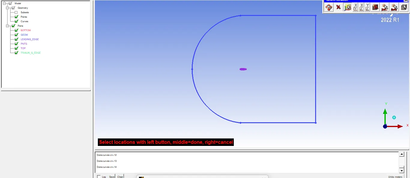
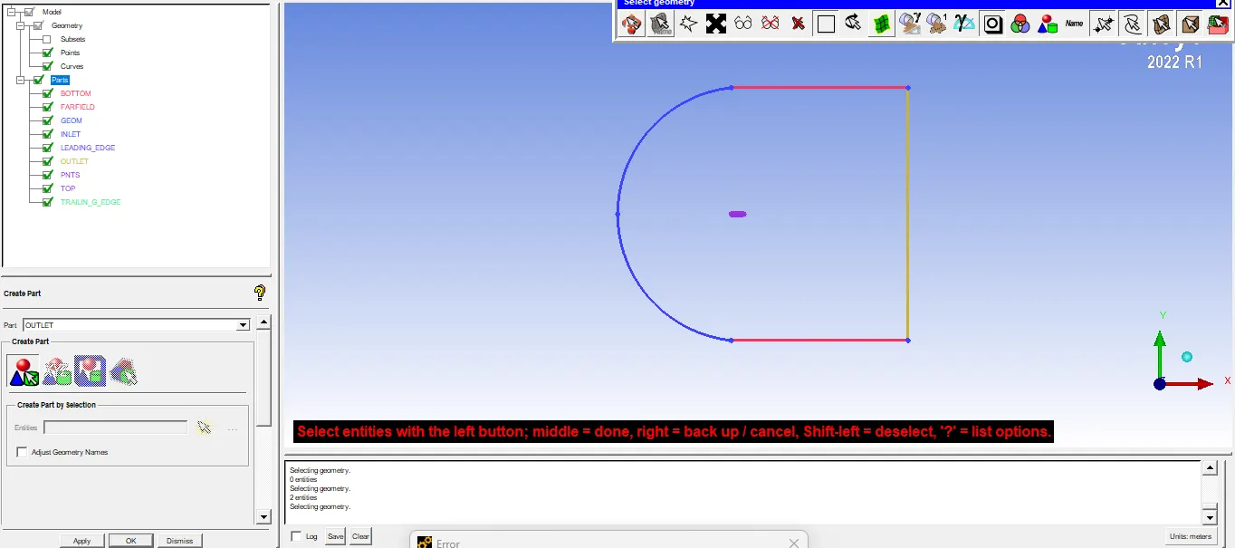
Thereafter the fluid conditions are defined with the domain as Inlet, symmetry and outlet.
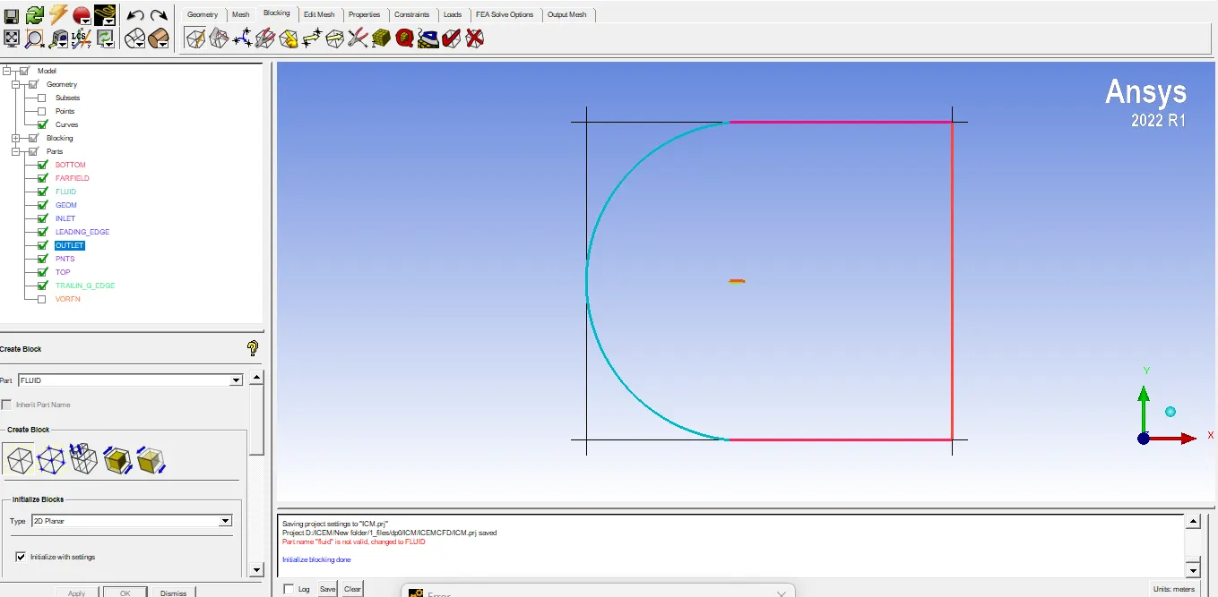
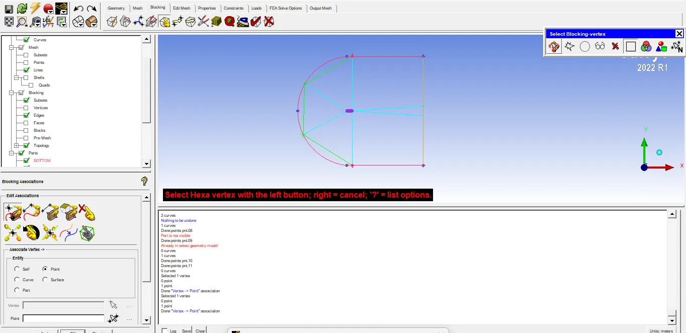
A 2D planar block is created as shown in the the figure.
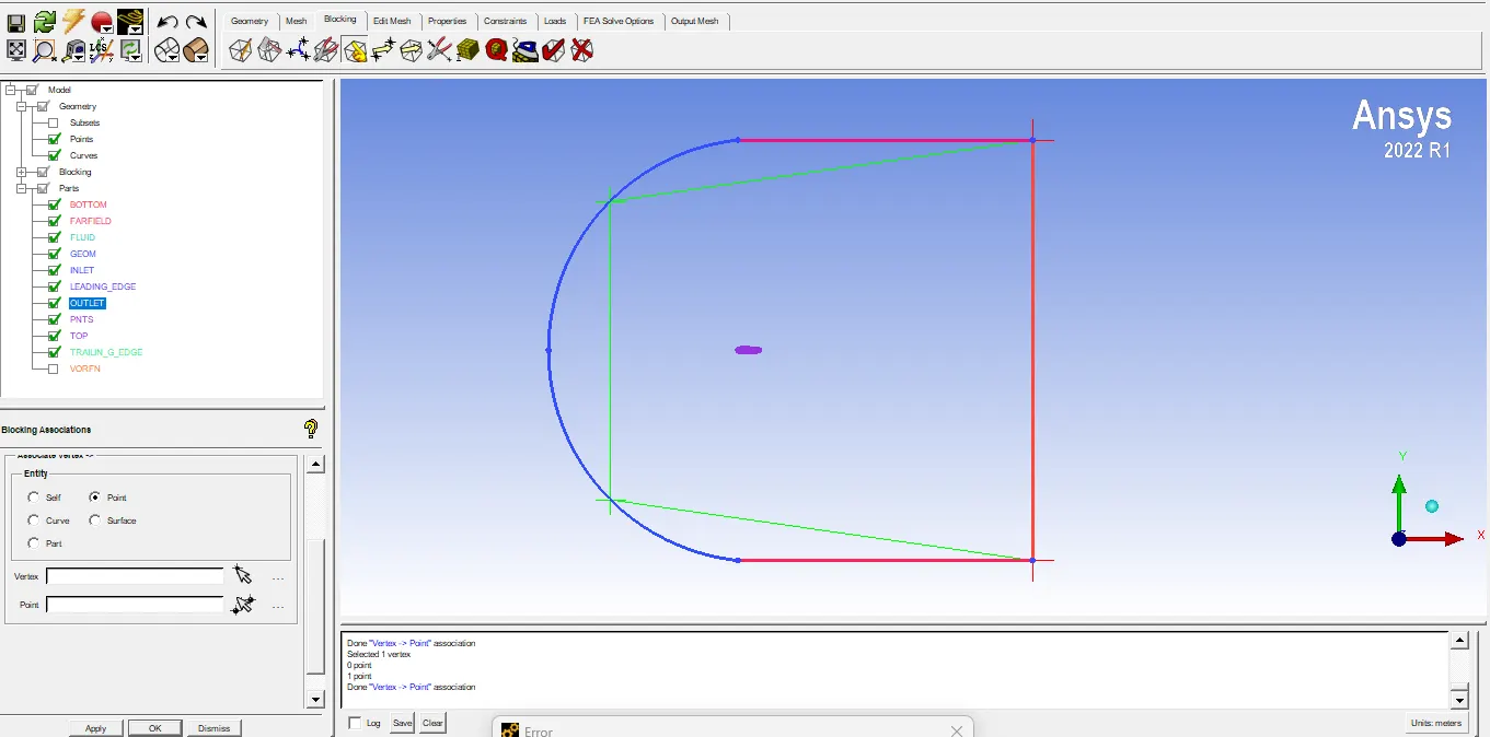
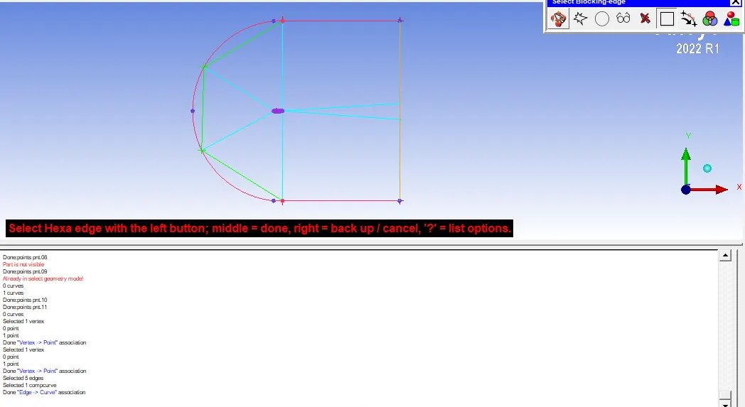
Once that is done the association of edges to the curves is done to map the physical domain on the computational domain thereafter the vertices are also associated with the airfoil surfaces.
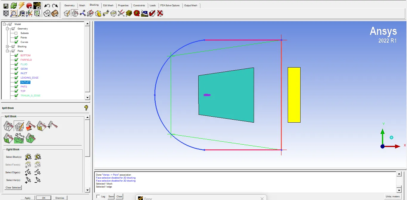
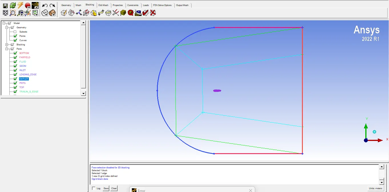
A splitting of block is done to create a new partition.
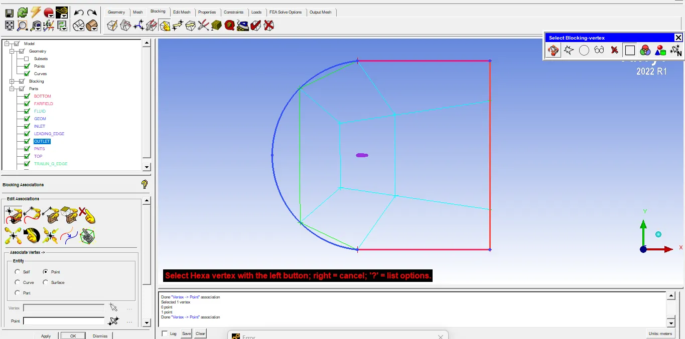
Mesh:
In the Pre-Mesh settings the edge parameters are defined to create the notes on the curves now with required spacing of 1e-05 and number of nodes the entire dominance divided into small grids as shown in the figure.
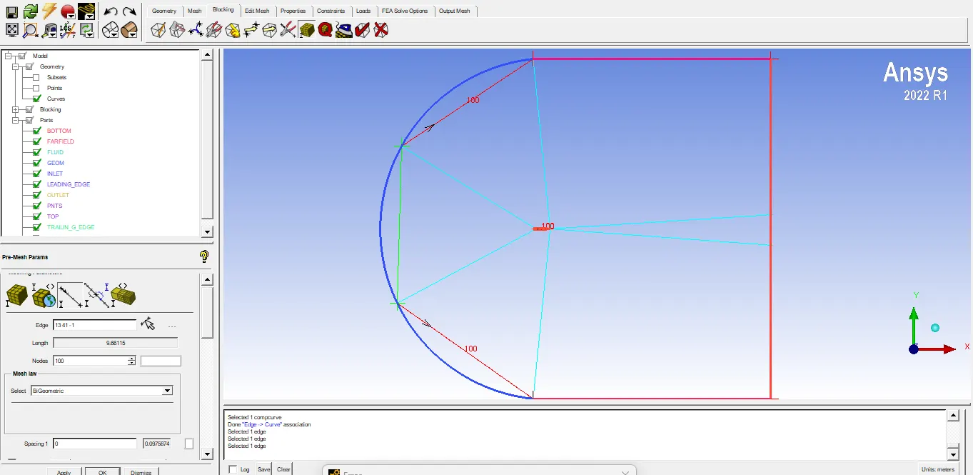
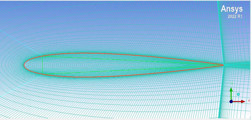
After setting up the PreMesh, the inner block of airfoil is deleted.
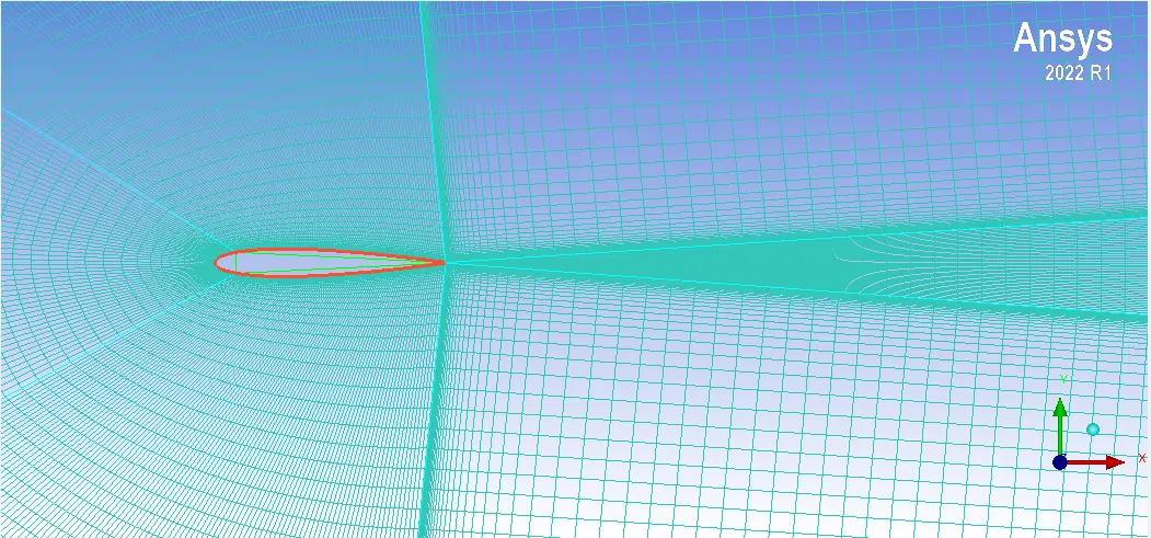
The above figure shows the computational mesh created for the incompressible flow case.
It is seen from the figure that the mesh is inclined after the trailing edge which is not suitable to capture the shock phenomena in case of compressible flow. So for that additional points are created on the curves and they are associated with the trailing edge points and are moved such that the mesh in that region is aligned with the trailing edge.
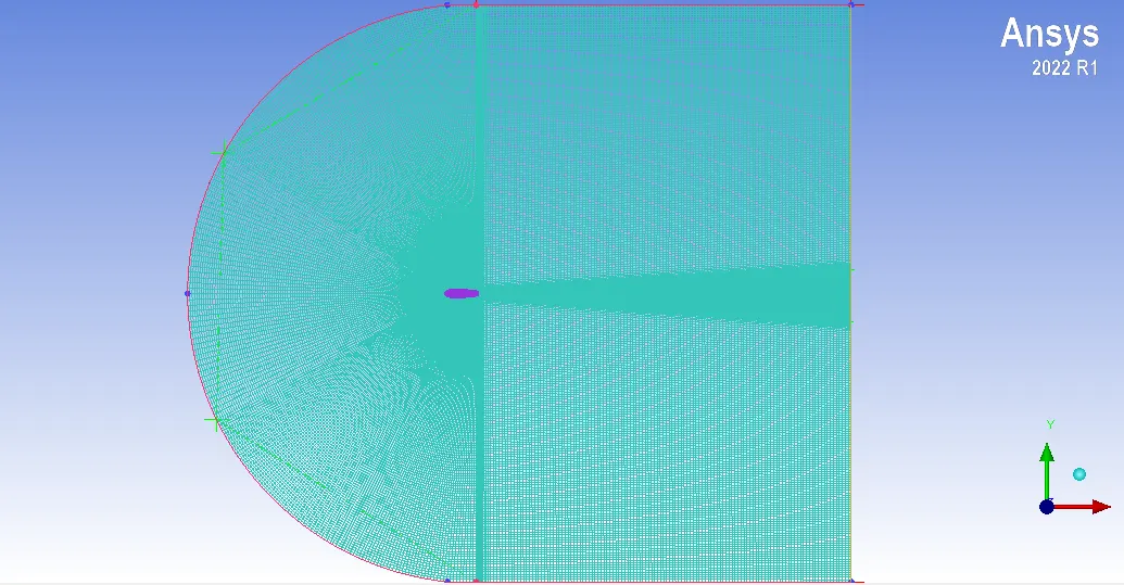
Lastly, the boundary conditions are defined in ICEM CFD and Mesh is written for output.
The Domain is set to 2D with total cells of 97626, and is imported to '.msh' file.
Solver Setup:
The velocity inlet conditions is set as per the angle of attack as shown;
| Velocity (m/s) | Angle of attack(degrees) | X compo. (m/s) | Y compo. (m/s) |
| 52 | 0 | 52 | 0 |
| 52 | 5 | 51.8 | 4.53 |
| 52 | 10 | 50.22 | 13.45 |
| 272 | 15 | 263 | 70 |
The Outlet is set as Pressure outlet as 0 Pa.
The airfoils walls are given wall conditions as the flow does not slip on the surface.
The report definitions are created for Lift and Drag coefficient.
The k-omega SST is considered for the viscous model as the boundary layer effects are of importance here.
In the solution, the Pressure Velocity scheme is kept coupled. Spatial Discretization which stores the discrete vales of scalar variables at cell centres is kept to Second order upwind for Momentum and Modified Turbulent Viscosity.
Contours and Plots:
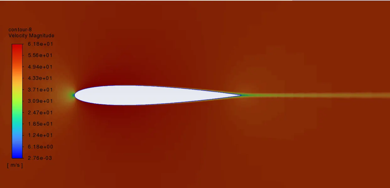
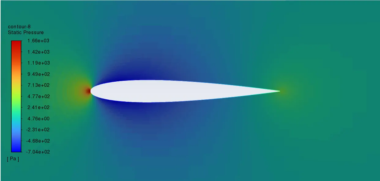
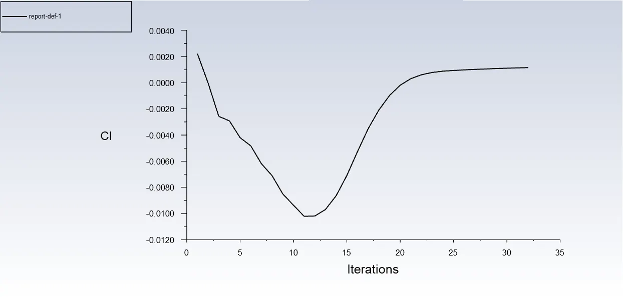
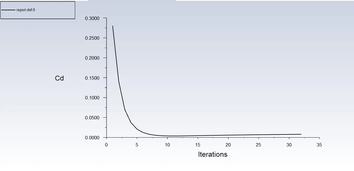
For 0 degree angle
1. Velocity Contour:
2. Pressure Contour:
3. Lift coefficient plot:
4. Drag coefficient plot:
For 5 degree angle
1. Velocity Contour:
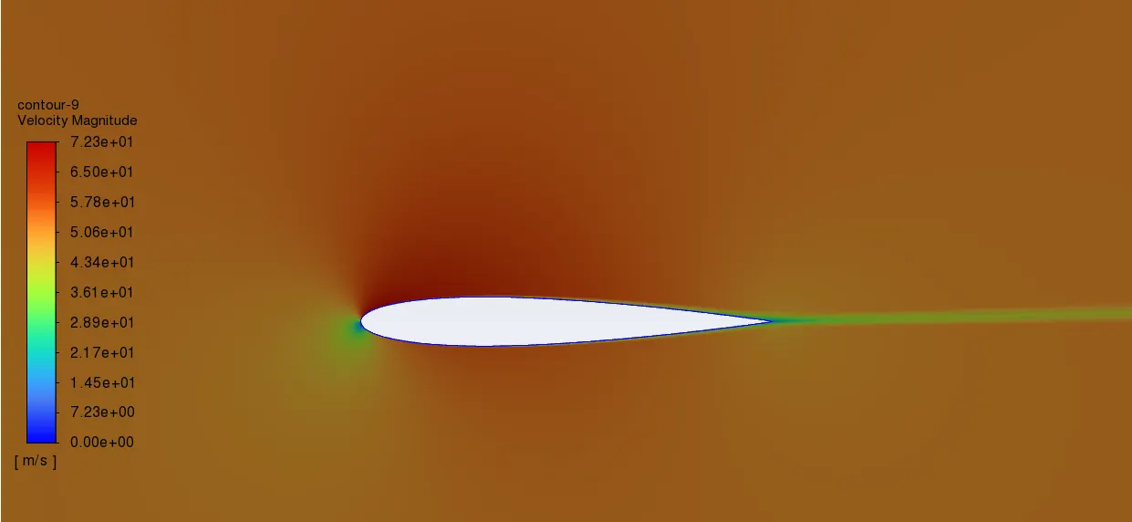
2. Pressure Contour:
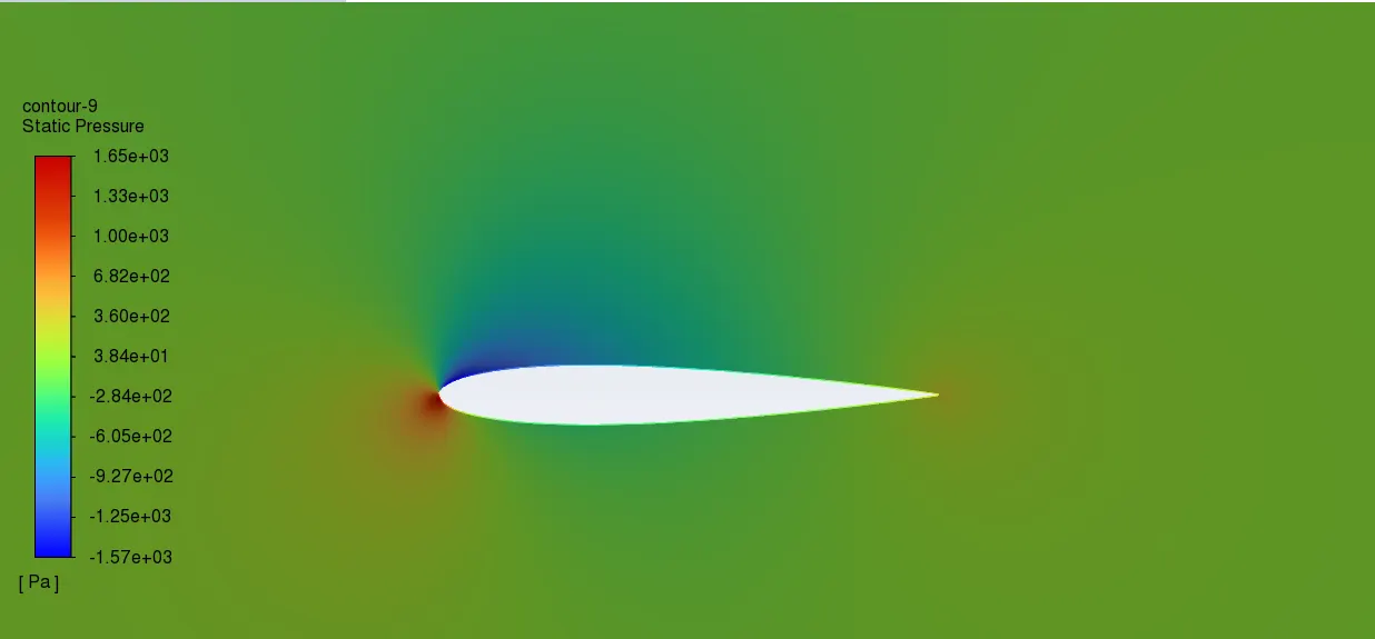
3. Lift coefficient plot:
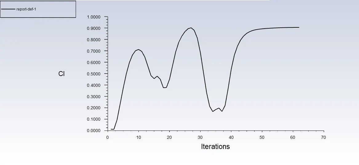
4. Drag coefficient plot:
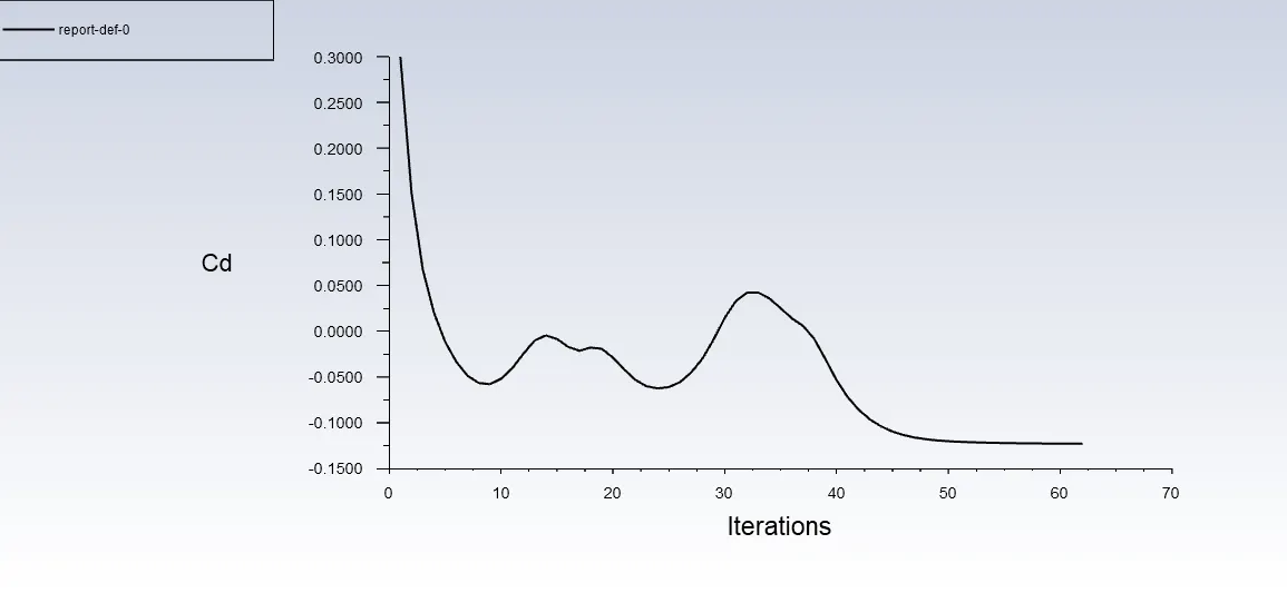
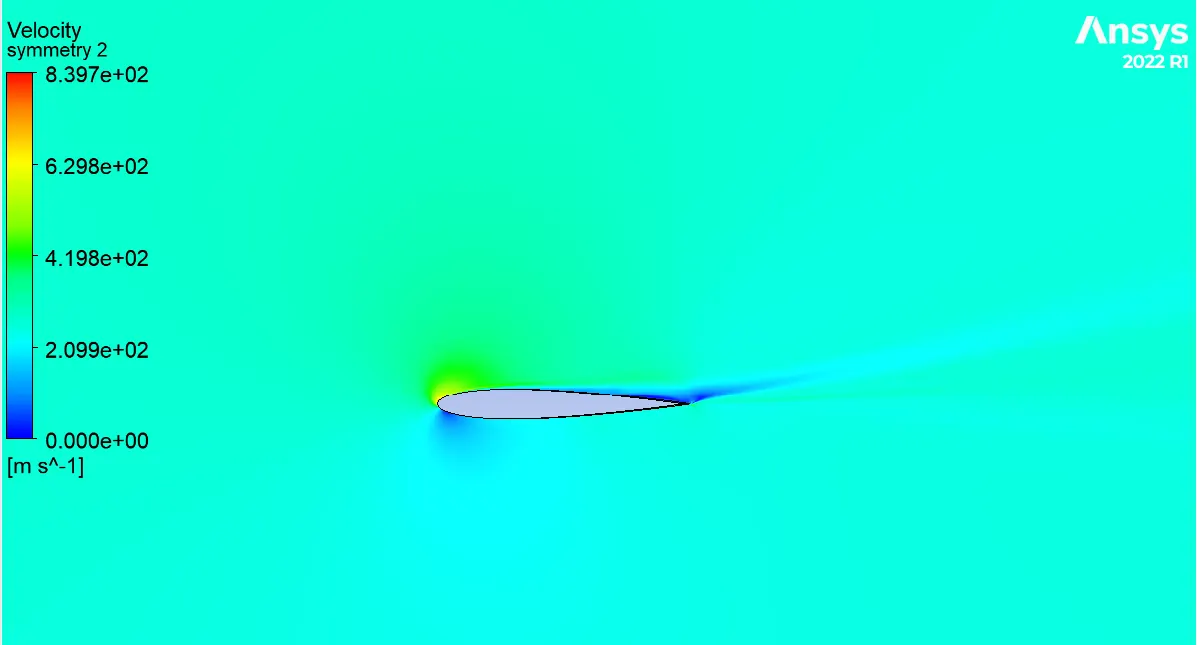
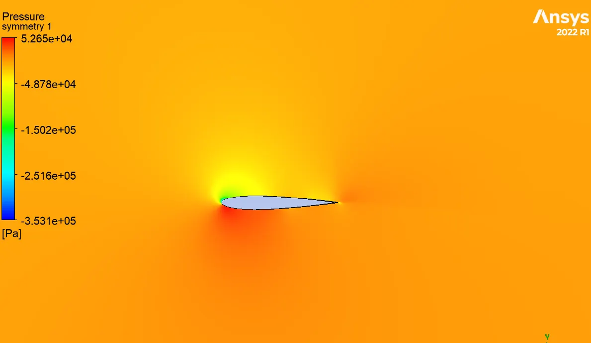
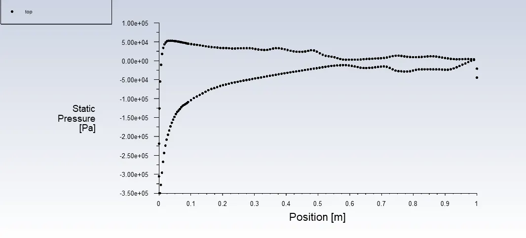
For 15 degree compressible flow;
1. Velocity Contour:
2. Pressure Contour:
2. Coefficient of Pressure against chord:
Variation in Lift and Drag Coefficient based on angle of attack:
| No. | Velocity (m/s) | Angle of Attack | Lift Coefficient(Cl) | Drag Coefficient(Cd) |
| 1. | 52 | 0° | 0.0011 | 0.0078 |
| 2. | 52 | 5° | 0.9051 | 0.1227 |
| 3. | 52 | 10° | 0.574 | 0.0462 |
| 4. | 272 | 15° | 1.46 | 0.24 |
Conclusion:
Here as seen from the values of table, the lift and drag are minimum for 0° as there is no difference in pressure on upper and bottom surface, also as this is a symmetric airfoil, net lift obtained is very negligble.
As the angle of attack is increased, the values of lift and drag coefficient gradually start to increase. the Lift-to-Drag ratio obtained here is around 7. Furthermore, by increasing the angle to 10°, the Lift-to-Drag ratio increases to 12 approximately. The angle of attack more than 12°-14°, can lead to stall and flow separation.
For the compressible case, flow separation is seen as the flow does not remain attaached at the trailing edge as of very low skin friction effects. Here the Lift-to-Drag ratio is somewhere around 6.