Week 4.2 - Linear Convection for varying timesteps

Week 4.2 - Linear Convection for varying timesteps

Aim : To create a function which considers the different values of time steps for a fixed set of parameters.

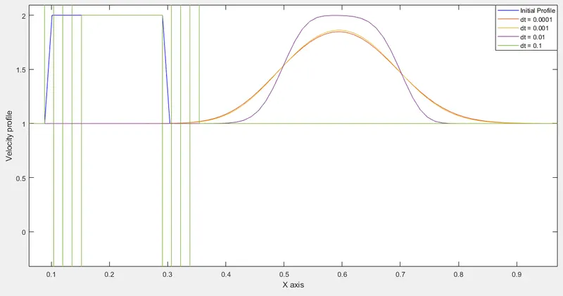
The program starts by defining the parameters as domain length, nodes, convection speed and the length is discretized as X-axis thru linspace command with 80 nodes, along with 'dx' as distance between two meshed points. Secondly, four different time steps are defined and it follows by creating a square shape velocity profile for nodes 9 to 24, having velocities 2m/s and 1m/s everywhere else. Upto this part, the initial velocity profile is plotted.

Now for accounting the value of four different time steps, a function is created which has variables as time step, initial velocity, number of nodes, convection speed and dx. Here the steps for the loop are defined for each value of dt. Thereafter a space loop is created for general step equation for n number of nodes and this is again looped in a specified time loop for each value of dt. Furthermore, this time step function is fitted in the main program which has all else parameters fixed but only the value of dt as changing. In order to illustrate the variation in velocity profiles, hold on command is used which captures all the curves in a same and single plot.

Program:

%1D Convection equation
clear all
clc

%inputs for equation
L=1;  %domain length in metres
n=80; %total nodes (current)
c=1;  %convection speed in m/s

%calculation
x = linspace(0,L,n);
dx=L/(n-1);
dt = [1e-4 1e-3 1e-2 1e-1];

%Define start and end position of a square wave
n_start = 9;
n_stop = 24;

%B.C.s
u=1*ones(1,n)
u(n_start:n_stop) = 2
u(1)= 1;
% uold= u;
u_initial = u;


% Plotting the initial velocity profile
figure (1)
plot(x,u ,'b',DisplayName='Initial Profile');
xlabel("X axis")
ylabel("Velocity profile")
axis([0 1 0 2])

for i = 1:length(dt)
    u = time_step(dt(i),u_initial,n,c,dx);

    %Plotting the velocitie profiles
    figure(1)
    hold on  
    plot(x, u, DisplayName=['dt = ',num2str(dt(i))])
    axis ([0 1 0 2])
    legend
end

Function:

function[u] = time_step(dt,uold,n,c,dx)
u = uold
nt = 0.4/dt;

% Time loop
for k=1:nt
    %Space loop
    for i=2:n
        u(i)=uold(i)-(c*dt/dx)*(uold(i)-uold(i-1));
    end
    %update old velocities
    uold = u;
end

end

Variation in profiles as per change in Courant number

The CFL or Courant Number comes into picture where the problem is time marching; Explicit Methods, for stability, is dependent on the CFL Number and the Implicit Methods are not sensitive with the changes in Courant Number.

The CFL number is given as,
`CFL = c(Δt)/(Δx)`

where c = convection speed, m/s

`Δt` = time interval

`Δx` = grid size

Here the value of 'c' is fixed and is 1m/s and the grid size is dx, which for 80 nodes is 0.0126. Thus for each value of dt, following is noted;

`Δt`	CFL Number
0.0001	0.0079
0.001	0.079
0.01	0.79
0.1	7.9

From the above table it is clear that, for the values of CFL less than 1, the profiles are showing an approximate behavior, while, in case where the CFL number exceeds more than 1, no profile is observed(or seen a flat line), and there are oscillations present.