Week 2.1 - Air standard Cycle

Week 2.1 - Air standard Cycle

Aim : The given program is regarding calculating thermal efficiency of the Otto cycle and plotting four thermodynamic processes on a p-v diagram.

To begin with, the program starts by predefinition of Input variables, State variables, Engine's parameters, and follows up by calculating initial volume (v1) and clearance volume (v2) by defining Swept and Clearance volume by emprical relations.

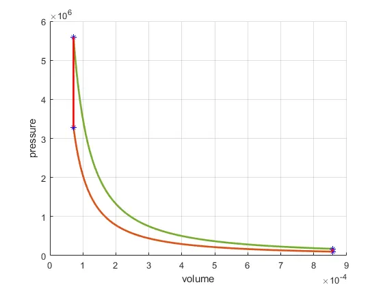
The state variables at stage 2, 3 and 4 can be evaluated using thermodynamic relations of the Otto cycle. Thereafter, the 4 states of the cycle are plotted using the 'plot command', however, in order to interconnect the 4 stages, the 'plot' command incorporating the specific volume variables and pressure variables cannot be used, else it will give a trapazoidal plane figure. So regarding that, the movement of engine components and the variation in the volume has to be taken into account.

Now, a 'theta' as a linspace which covers a range of angles(from beginning to end of crank rotations) with numerous intervals is defined and a function having input of components (bore, stroke and rod length, compression ratio and starting and ending crank angle) is created, which traces the Volume(V) as an output. Subsequently, the value of the variable 'V', is then defined by a complex relation, by simplifying into three terms. All the parameters here are assigned as a function named 'engine_kinematics', which when added to the program, gives out value of volume at isentropic compression, i.e. V_compression. With that, the value of pressure at the same stage (P_compression) is found by using the Ideal Gas law, considering the product of 'moles(n)' and "Gas constant (R)" as a 'constant_c' for the 1st process.

Similarly, 'V_expansion' as an output of the same function of 'engine_kinematics', is created at isentropic expansion process. Here, taking into picture, state variables of stage 3, 'P_expansion' is solved out using the same gas law. The "V_compression, P_compression" and "V_expansion, P_expansion" are assigned after the state variables 2 and 3 respectively, which means they hold the magnitude of volume and pressure at that instant as a function of 'engine_kinematics'.

Likewise, the plotting of them using "hold on" command, which prevents the overlapping of plots, is done which depicts the thermodynamic nature of the curves, based on the precreated plots (of 4 stages) and on the basis of variation of pressure and volume at compression and expansion processes respectively, with appropriate line width and color. Also, for connecting plots 2 and 3, and 4 and 1 linearly, the variables [v2 v3], [p2 p3] and [v4 v1],[p4 p1] are assigned as arrays. Additionally, using 'xlabel' command, X axis is titled 'volume' and Y axis, with 'ylabel', 'pressure', with grid.

Furthermore, the value of expansion ratio (e_r) is calulated using derived formula and the cycle efficiency (n) can be worked out using provided formula,(which comes around 96.82% for current case).

% Input variables
gamma = 1.4
t3 = 2300

% State variables
p1 = 101325
t1 = 500

% Engine Geometric parameters
bore = 0.1;
stroke = 0.1;
con_rod = 0.15;
cr = 12;

% Swept and Clearance volume
v_swept = (pi/4)*bore^2*stroke;
v_clearance = v_swept/(cr-1);

v1 = v_swept + v_clearance
v2 = v_clearance

% State variables at 2
p2 = p1*cr^gamma; 
t2 = p2*v2*t1/(p1*v1)

constant_c = p1*v1^gamma;
V_compression = engine_kinematics(bore, stroke, con_rod, cr,180,0);

P_compression = constant_c./V_compression.^gamma;

% State variables at 3
v3 = v2
p3 = p2*t3/t2

constant_c = p3*v3^gamma;
V_expansion = engine_kinematics(bore, stroke, con_rod, cr,0,180);

P_expansion = constant_c./V_expansion.^gamma;

% State variables at 4
v4 = v1
p4 = p3*(v3/v4)^gamma

figure(1)
hold on
plot(v1,p1,'*','color','b')
plot(V_compression, P_compression, 'linewidth', 2)
plot(v2,p2,'*','color','b')
plot(v3,p3,'*','color','b')
plot(V_expansion, P_expansion, 'linewidth', 2)
plot(v4,p4,'*','color','b')
plot([v2 v3], [p2 p3], 'linewidth',2, 'color','r')
plot([v4 v1], [p4 p1], 'linewidth',2, 'color','r')
xlabel('volume');
ylabel('pressure');
grid on

% Expansion ratio (e_r = v4/v3)
e_r = 12

% Cycle efficiency (n)
n = 1-(1/(e_r^gamma - 1))