Week 8- Moving zones approach in Fluent

Week 8- Moving zones approach in Fluent

Basically there are two approaches that can be utilized to model the "Moving Zones/Frames" in Ansys Fluent.

There are discussed as follows:

1. Moving Reference Frame

• Here the frame will be in motion and the mesh topology will remain the same
• There is no change in the Control Volume of a system
• It is a steady phenomena
• It is suitable when unsteadiness is not important

2. Moving Mesh Approach

• Here the mesh will be moving and the topology will also change with time
• Control volume will change with time
• Moving mesh approach (with Transient case) is appropriate to consider when required to capture unsteadiness.

The following problem deals with simulating a turbomachinary component with "Moving Reference Frame" approach with steady state case.

Problem Specification:

• Geometry: Turbomachinary component
• Total blades: 10
• Dimensions: Chord of 0.6 m, spaced by 36 degrees
• Load conditions: No Pressure difference, Inlet and Outlet at atmospheric condition
• Blade Velocity: 250 rpm
• Flow Regime: Assumed to be turbulent

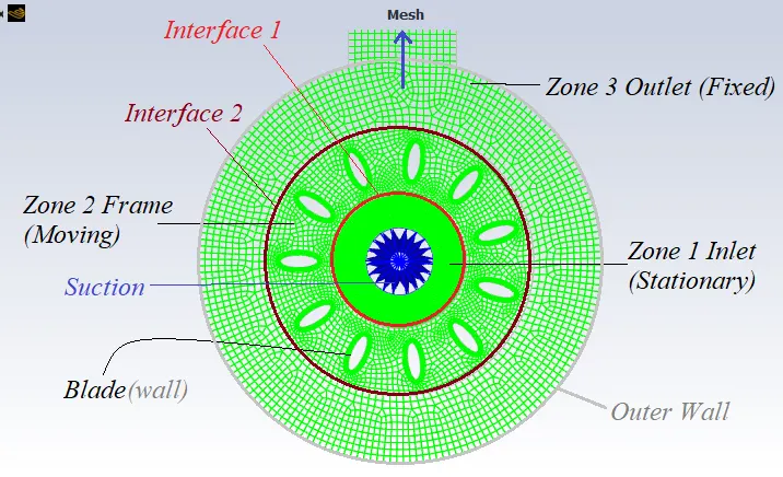
To begin with, the Domain 1 mesh file with other two are appended as a case in Fluent. Below figure represents the geometry details.

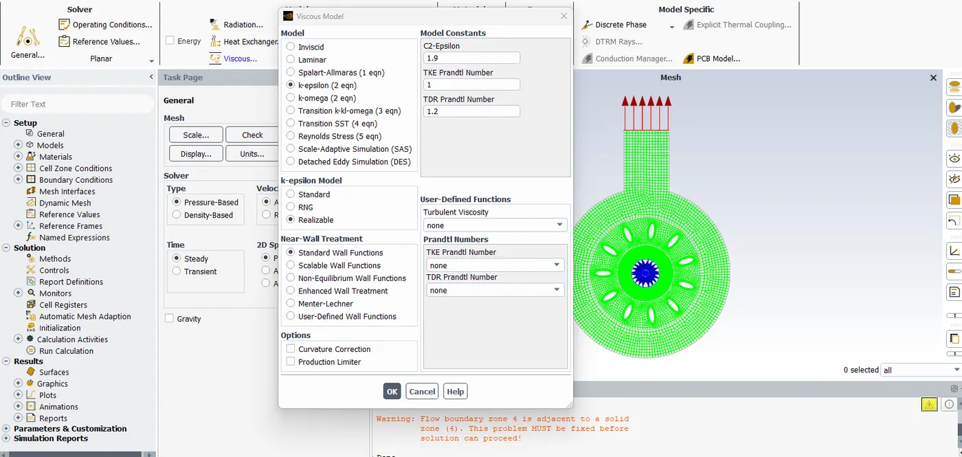
Since the geometry is moving, the viscous model is set to k-epsilon Realizable with Enhanced Wall treatment.

The material is set to 'Air' with standard atmospheric conditions.

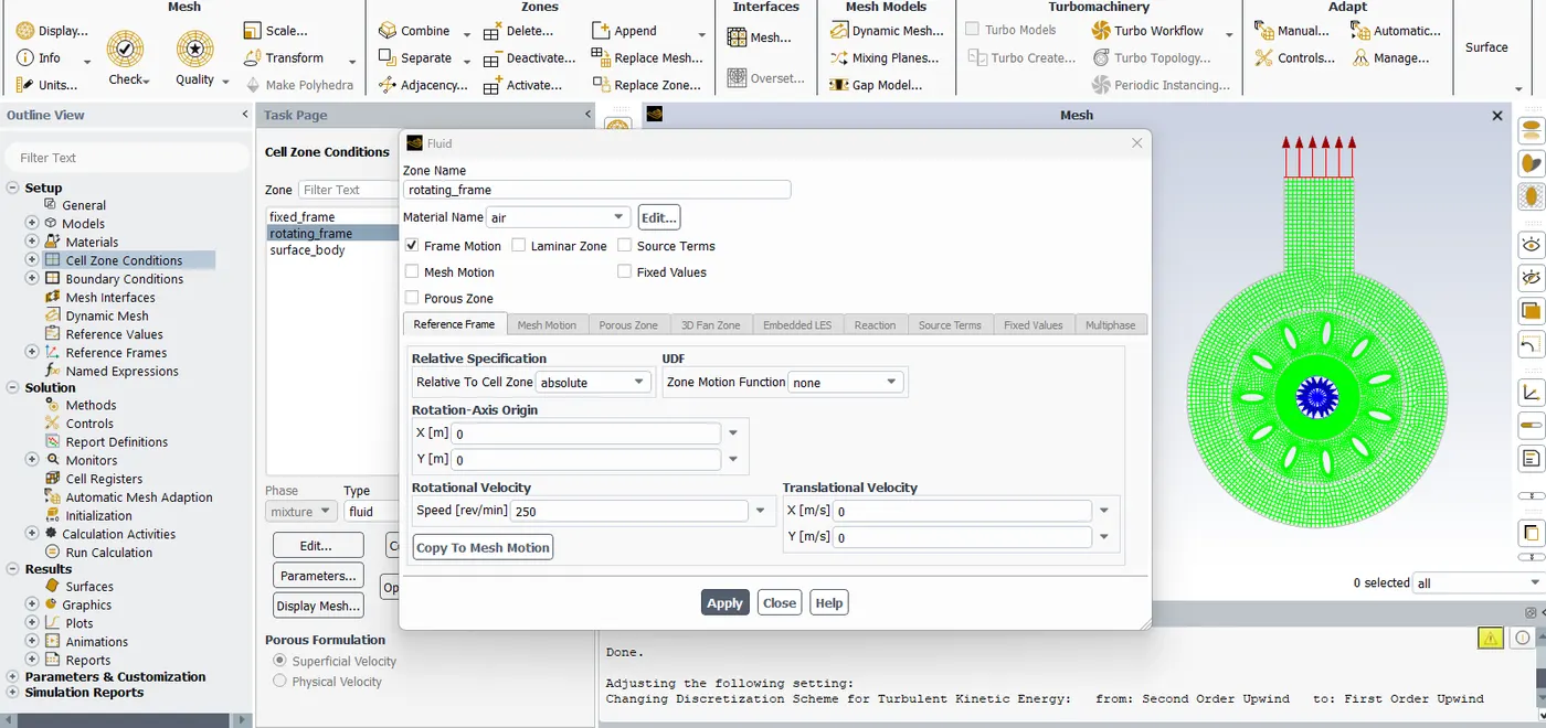
In order to flow take place inside the geometry, the Cell zone condition for Zone 1, 2 and 3 is set to 'Fluid'.

The Inner and Outer, i.e, Zone 1 and 3 are kept stationary with no moving frame, whilst, for the Zone 2, the "Frame Motion" is enabled, and an input angular velocity of 250 rpm is provided.

With regards to the Boundary Conditions,

• The airfoil is kept as moving wall, with motion related to adjacent cell zone, i.e. Zone 2, since its locations is on the rotating component.
• The 'Frame3_inner' is the interface of Zone 2 and 3, as the fluid will have to move out of the Zone 2, its condition is kept as 'interface'.
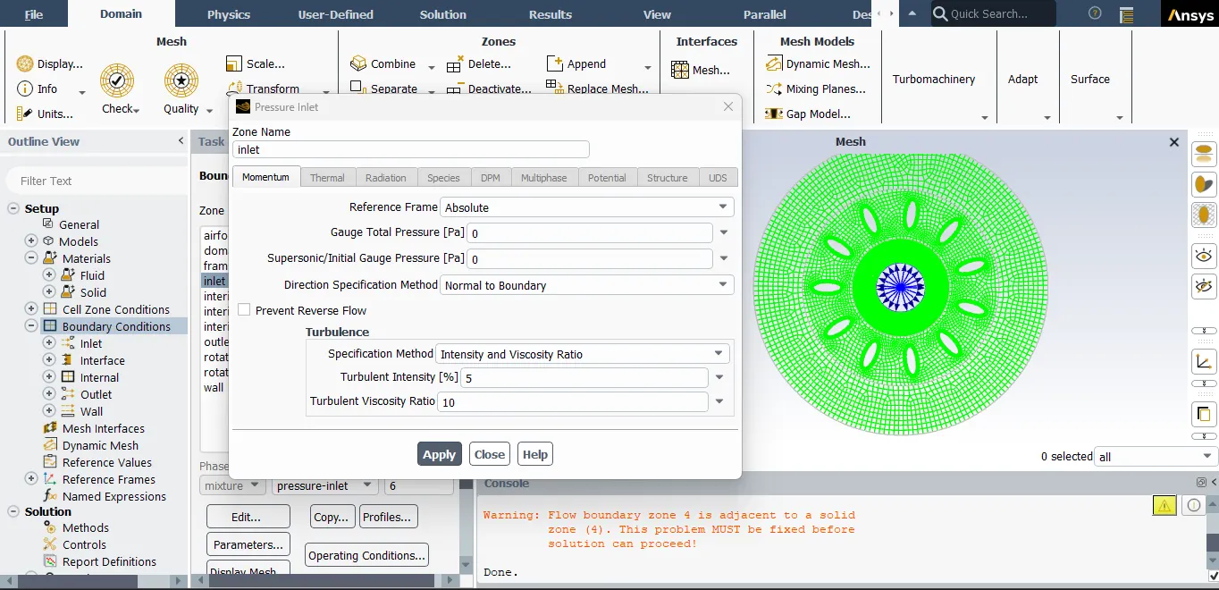
• Since there is no pressure difference between inlet and outlet, the Inlet boundary condition is set to 'Pressure Inlet' with Gauge pressure of 0 Pa and the interior sections are set to interior.

• As mentioned earlier, because of no pressure difference, the Outlet is set to Pressure Outlet with Gauge pressure of 0 Pa.

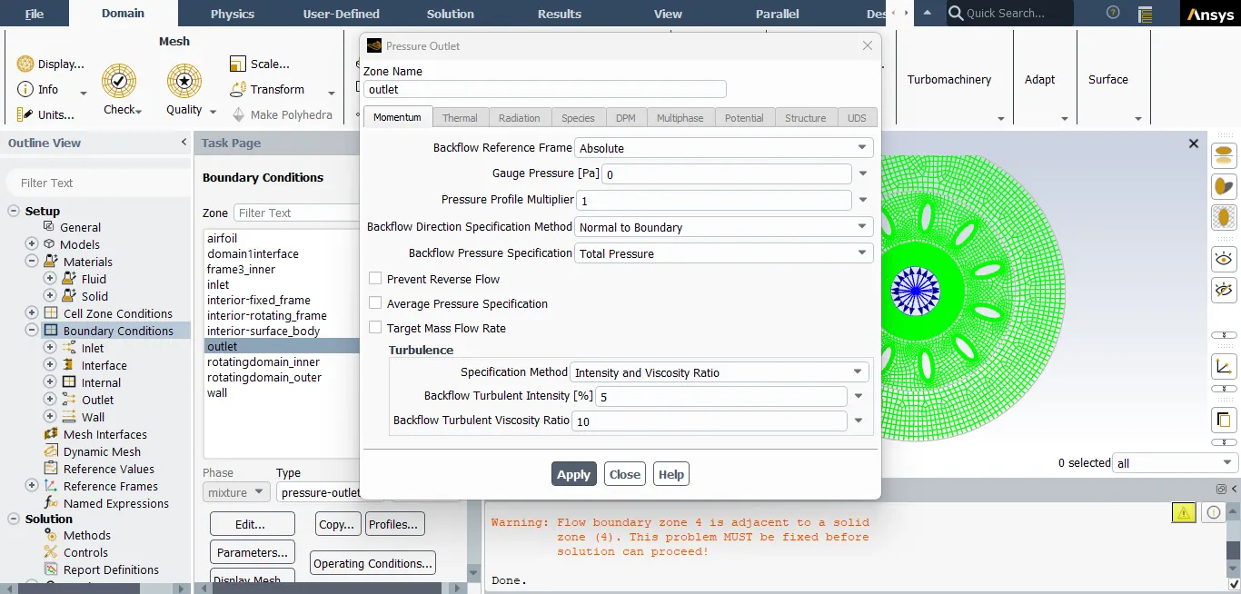
• Now as the fluid needs to pass thru the domains, the rotating inner and outer domains are set to interface.

Mesh Interface:

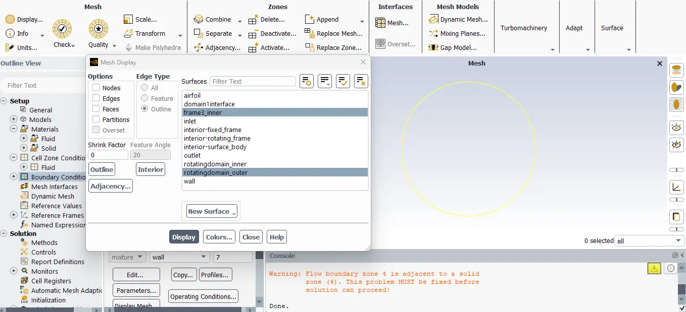
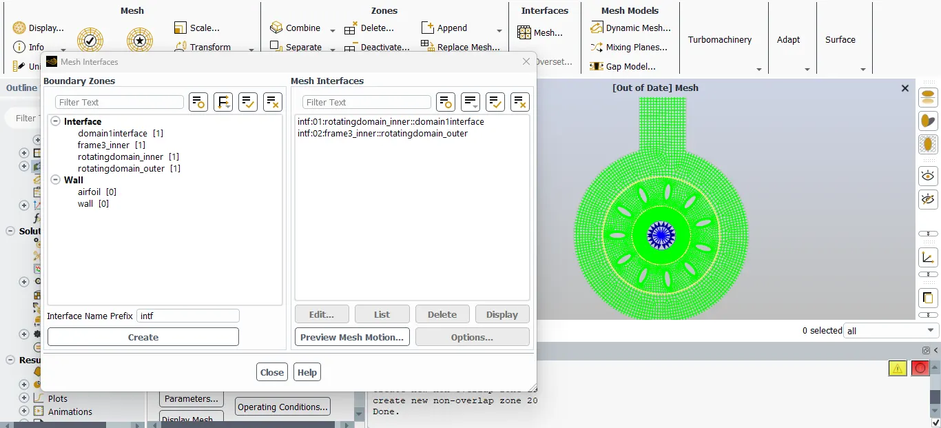
The 'rotatingdomain_outer' and 'Frame3_inner' are overlapping, so they need to be set as Mesh interfaces. The same will be applicable for the 'rotatingdomain_inner' and 'domain1interface'.

Reference Values:

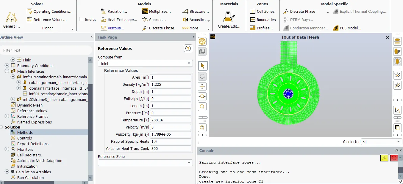
The Reference Values are to be calculated from the Inlet.

Solution Method:

The Pressure Velocity scheme is set to 'Coupled' as this algorithm provides more advantages over the Pressure-based segregated algorithm.

For spatial discretization, convection fluxes set to predict with Second order upwind scheme. So the scheme is used for "Turbulent Kinetic Energy" and "Specific Dissipation Rate".

The minimum Courant number is set to 10.

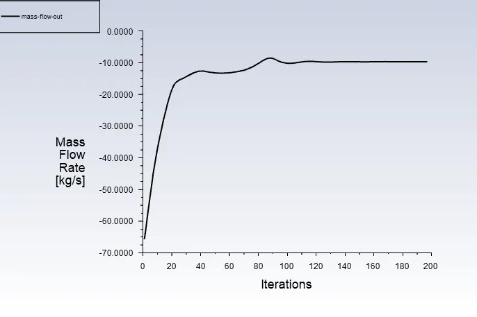
For the solution, the Outlet Mass Flow rate based on provided conditions is monitered.

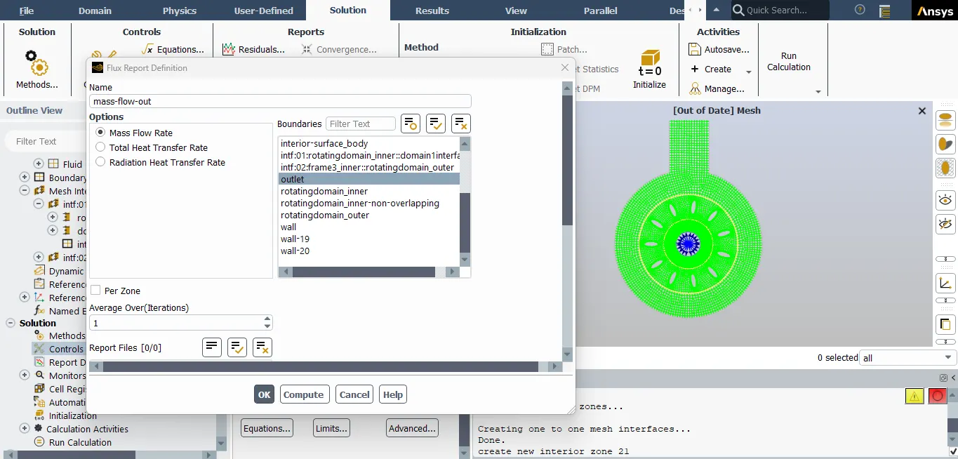
With Hybrid initialization. the initial values of the solution are guessed by the solver based on the given boundary conditions and the solution is ran for 500 iterations.

Results:

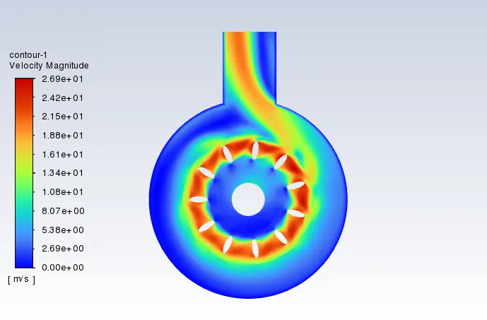
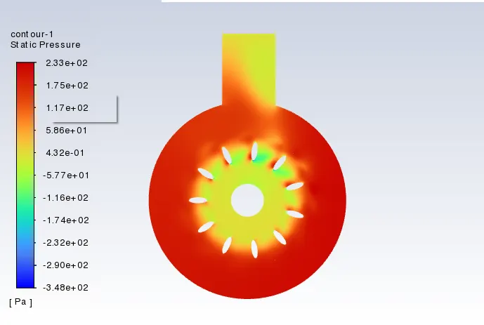
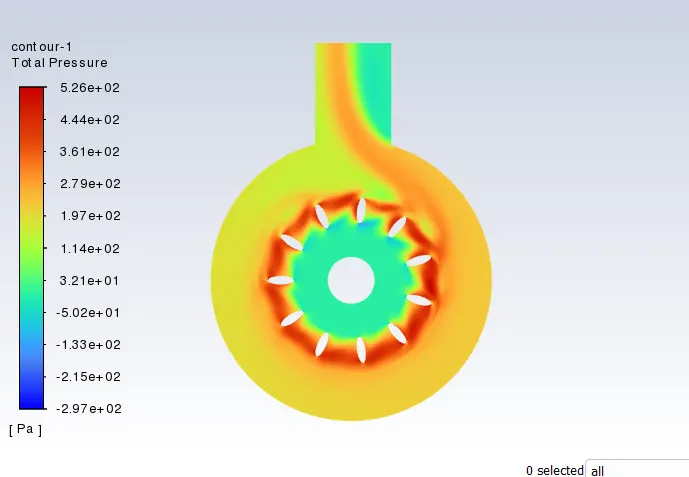
The below contours show the variation in Velocity, Pressure and Total Pressure.

1. Variation in Velocity

2. Variation in Static Pressure

3. Variation in Total Pressure

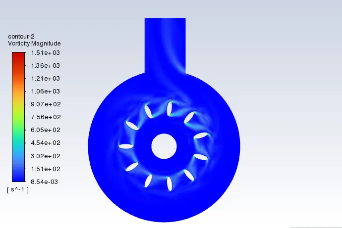
4. Variation in Vorticity of fluid

Plots:

Outlet mass flow rate:

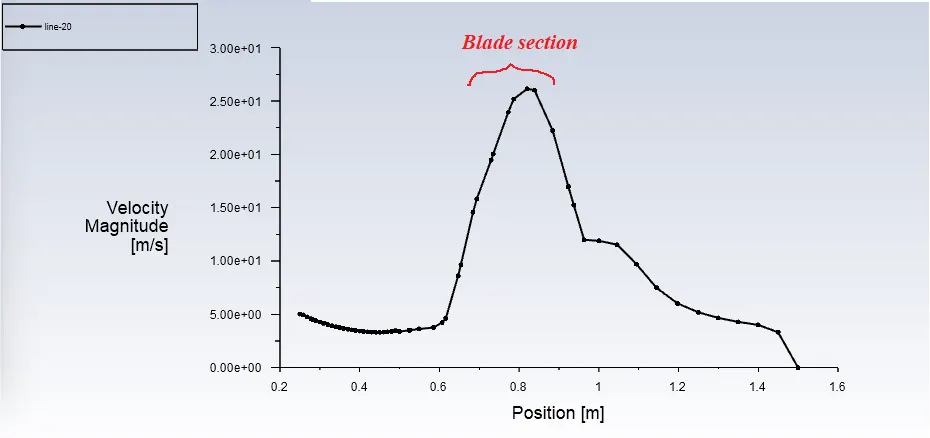
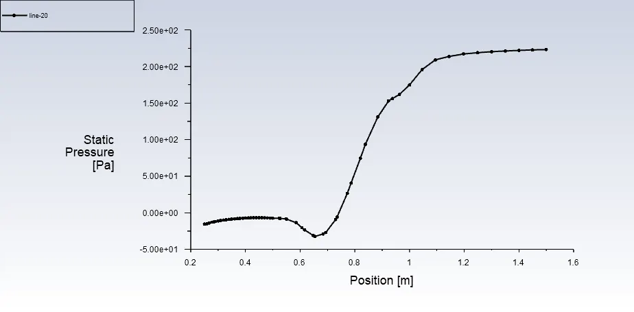
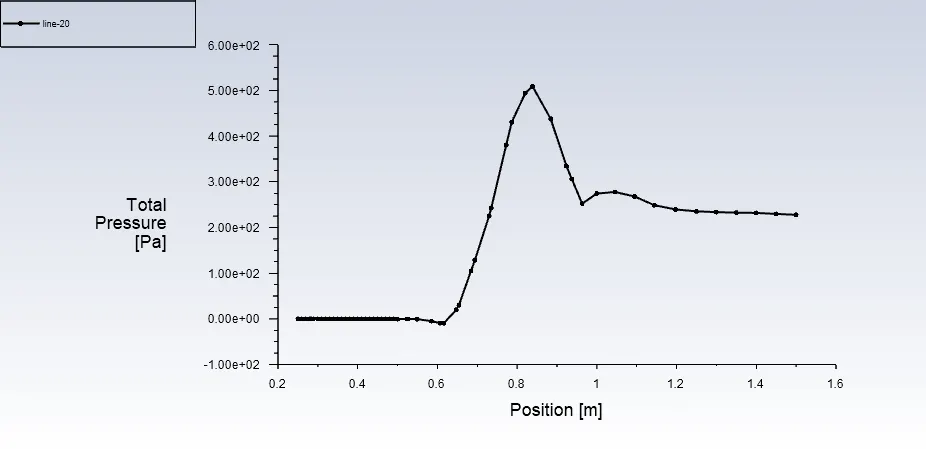
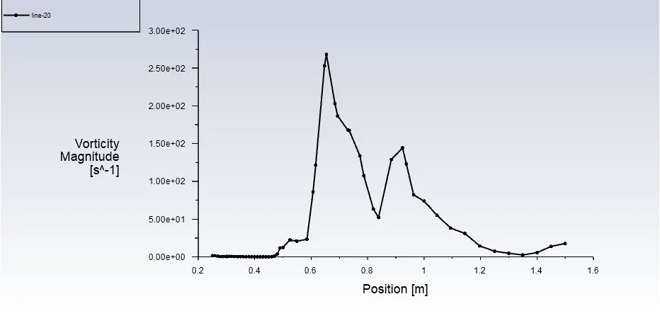
A line of 1.5m is created in x direction to visualize the variation in flow quantities in radial direction.

1. Radial Variation in Velocity

2. Radial Variation in Static Pressure

3. Radial Variation in Total Pressure

4. Radial Variation in Fluid Vorticity

Conclusion:

For the Moving frame problem, with a steady case setup, the maximum variation is seen at the blade section where the airfoils are moving and while moving outwards the velocity drops as of the diffuser section and simultaneously there is a rise in static pressure.

For the total pressure, as the quantity involves dynamic pressure as well, so at the rotational section, there is a rise in total pressure too, but specifically due to `rhov^2` term. Moving outwards, the total pressure is more than that of the inlet. The exit mass flow rate is roughly about 12 kg/s`

The plot and contour of the vorticity represents that there is significant amount of fluid swirling at the front and end section of the blade where the fluid leaves the zone 2.