Week 7 - Simulating Fluid Sloshing effect inside a Gear-box

Introduction to GUI based CFD using Ansys Fluent

Week 7 - Simulating Fluid Sloshing effect inside a Gear-box

Dynamic meshing:

The application of Dynamic meshing comes into use when the domain (or say the structured grid) is changing with time because of motion. The motion here can be linear or rotational based on which the calculation is done by solver using a User defined function. Initially a mesh needs to be provided and with each time step considering the transient simulation, the mesh is updated at its new positions. In present case the angular motion is defined planar. Dynamic mesh can be suitable when the geometry is in motion and influence the region around it. Typical examples could include the movement of air around flapping wings of a bird, collision of bodies inside fluid, motion of turbine rotors, flow over an oscillating airfoil, simulating moving pistons and fuel flow, etc.

Sloshing effect:

Model/Geometry has to be assigned with moving (here two gears) and non-moving regions. To account with 'slosh', it is liquid movement with hydrodyamic forces and moments due to motion of parts that are in contact with liquid in presence of gravity. With the movement of container, assuming that it is in motion and as of inertia, there are oscillations and makes motion of liquid unsteady. If there are oscillations in liquid above a certain frequency, it may make the maneuvering of a vehicle which carries the fluid difficult because of high impact pressure and loads. Extensive of these loads can also damage the structure.

User-defined function:

With use of UDF, it becomes easy to load parameters like custom boundary conditions and loading up parameters like Dynamic mesh, multiphase flows, etc. in the Ansys Fluent.

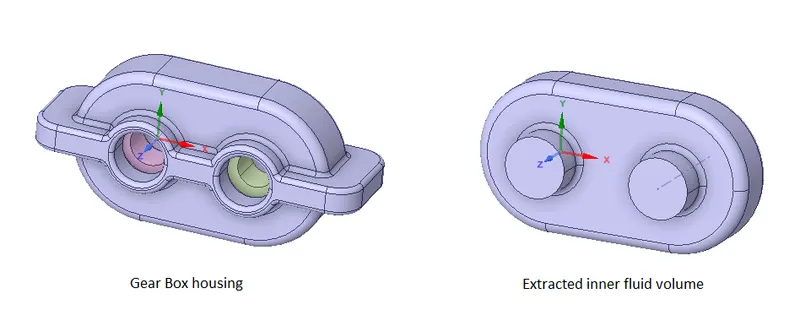
The present project deals with simulating the fluid sloshing inside a gear box. A CAD model of 3D gear box housing is loaded in Spaceclaim where the fluid volume (3D) is extracted, part is split and a two dimentional gears' rotation plane is extracted from it to create a 2D domain.

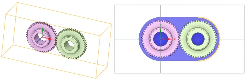
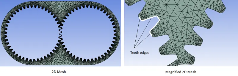
In the mesh module, the named selections of both the gears, as edges of teeth are made as "left gear" and "right gear", and then mesh is generated.

Fluent Setup:

Current setup goes with Pressure based solver as of low velocity of working fluid and Transient analysis is preferred, as it solves and better captures the flow and can be used to run at smaller time steps. Smaller time steps are required to observe the variations in quantities more accurately. Gravity is enabled and viscous model is selected as k-epsilon with enhanced wall treatment option.

In Ansys Fluent, the "Multiphase Model" with "Volume of Fluid" method is enabled. The VOF method is a surface-tracking technique applied to a fixed (Eulerian) mesh (in backgroud). It is used for two or more immiscible fluids where the position of the interface between the fluids is of interest. With the Euler-Langrangian approach, the Lagrangian discrete phase model follows the Euler-Lagrange approach. The fluid phase is treated as a continuum by solving the Navier-Stokes equations, while the dispersed phase is solved by tracking a large number of particles, bubbles, or droplets through the calculated flow field.

Implicit VOF formulation is chosen as with Explicit one, the CFL criteria gets violated sometimes with increase in Courant number. As far as working fluid is concerned, for the first part, air and water and in second, air and n-heptane(liquid), with the immersion depth of 20% and 30% for both the cases.

Material properties:

Material	Densitykg⋅m-3">kg⋅m−3��⋅�-3	Viscositykg⋅m-1⋅s-1">kg⋅m−1⋅s−1��⋅�-1⋅�-1
Air	1.225	0.0000181
Oil	889	1.06
Heptane	684	0.000409

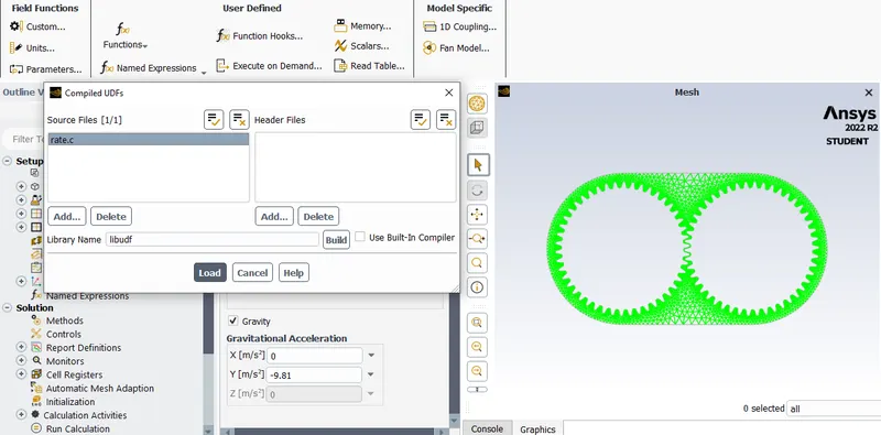
Thereafter, the UDF file is added, build and loaded to define the motion of two gears, which is given by;

#include "udf.h"

DEFINE_CG_MOTION(right_motion, dt, vel, omega, time, dtime)
{
	vel[0] = 0.0;
	vel[1] = 0.0;
	vel[2] = 0.0;

	omega[0] = 0.0;
	omega[1] = 0.0;
	omega[2] = 2.0e2; /* [rad/s]*/
}
DEFINE_CG_MOTION(left_motion, dt, vel, omega, time, dtime)
{
	vel[0] = 0.0;
	vel[1] = 0.0;
	vel[2] = 0.0;

	omega[0] = 0.0;
	omega[1] = 0.0;
	omega[2] = -2.0e2; /* [rad/s]*/
}

UDF explanation:

Here the angular velocities for both the gears is given, (negative of one with anticlockwise), with the relation and value of angular velocity as 200 rpm,

ω=2⋅π⋅N60">ω=2⋅π⋅N60�=2⋅�⋅�60, the value of N = 6000π">6000π6000�= 1910 rpm, which is 31.84 rps

In the Dynamic meshing method, the centre of rotation for the left and right gear is given as (0,0) and (0.115,0) metres respectively.

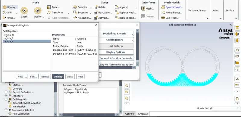
Before patching, the cells in the fluid region have to be defined and that is done by marking cells as co-ordinates in X and Y directions for defining the depth of liquid. Since there is no inlet, outlet present in the problem, the Hybrid initialization is done with constant pressure. Patching is done to assign different values of particular variables (or phases) into different cells. Here value of volume fraction to two different fluids is assigned to the zone created with 20% and 30% of liquid immersions.

Following are the co-ordinates for percent of liquid immersion:

For 20%:

	Min	Max
X	-0.0547	0.1697
Y	-0.085	-0.0395

For 30%:

	Min	Max
X	-0.0624	0.177
Y	-0.078	-0.0255

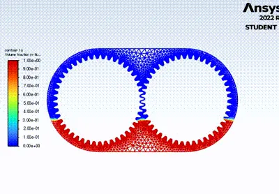
The initial contours for the multiphase simulation is as;

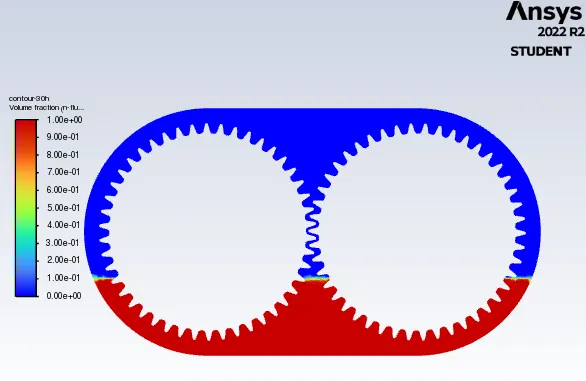
Considering the settings till now, after certain iterations the error of "Negative cell volume detection" comes up. This means that the CFL criteria is violated. The Courant Number is given by;

C=u⋅dtdx">C=u⋅dtdx�=�⋅����

where u = flow velocity, m/s

dt = time step size, seconds

dx = cell size. metre

In order to solve the error, cell size should be increased thereby making mesh coarse and by reducing the time step size.

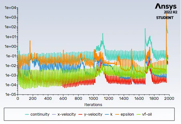
The "Floating point exception" error is encountered when the solution diverges. So as its solution, the time step should be decreased, for current case it was kept 0.0001s and Implicit solving scheme is preferable.

Apart from it, in the Dynamic Mesh settings, the Smoothing is done to deform the boundary layer while the mesh is moving and Layering, adds or removes layer from the moving boundary. With 'Remeshing', the minimum and maximum length scale of the mesh's deformation can be customized, here the min. scale is kept 0.0003 and maximum, 0.0004.

The simulation is ran for the following cases;

CASE 1 : 20% Immersion, Fluid - Engine oil

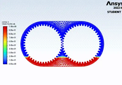
CASE 2 : 30% Immersion, Fluid - Engine oil

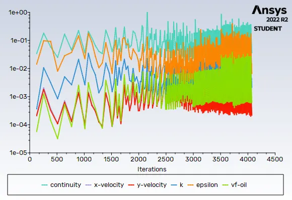
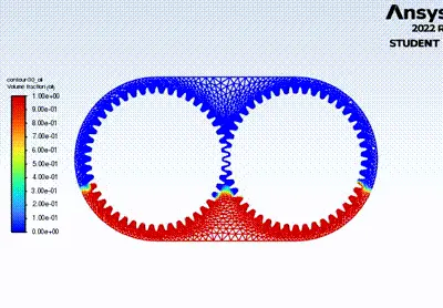
CASE 3 : 20% Immersion, Fluid-n-heptane (c7h16)

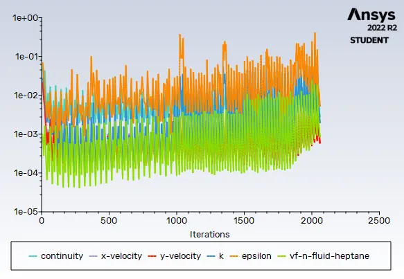
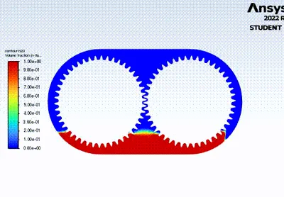
CASE 4 : 30% Immersion, Fluid-n-heptane (c7h16)

Conclusion:

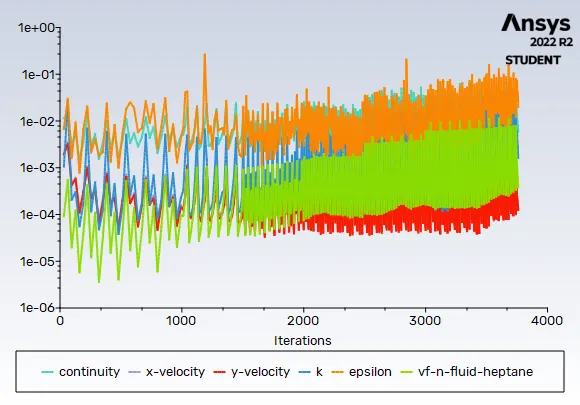
As seen from the computed residuals, the value of velocities in x and y directions, along with viscous model's and continuity equation's convergence, those parameters are completely fluctuating, as the quantities do not remain steady in there and keeps on changing due to sloshing effect.

The rate of mixing of n-heptane and air, via sloshing is more as the density of n-heptane is lower than that of the oil. Secondly the sloshing takes place faster in case of liquids that are 30% immersed.

Additionally, as compared to 20% of immersions, little more number of gear teeth are in contact with the lubricants, this implies that lubrication and sloshing on the surface of teeth starts some time before in 30% immersions, particularly in case of n-heptane and air. Furthermore, the layer of oil film that forms on the gear teeth while being in rotation, as of high viscosity, remains sticked. This is critical as the generated friction due to the rubbing action remains in control and the wear and tear of in contact moving parts is less.