Week 4.1 - Linear Convection for varying number of nodes

Week 4.1 - Linear Convection for varying number of nodes

Aim - To describe the behaviour of 1D Linear Convection equation for a varying number of nodes.

The program starts by defining the input parameters like domain length, nodes, convection speed and time step size and follows by creating a mesh by linspace 'command'. Secondly, to create a square shaped initial velocity profile the start and the end points, for total 20 nodes, are selected as 3 and 6 respectively. At the entire points the velocity value is assigned as 1m/s while for nodes, whilst at 3 and 6 where the mesh value is 0.1 and 0.3, approximately, the velocity is given digit 2m/s. Upto this point, a subplot is generated which illustrates the initial velocity profile.

In order to implement the backward differencing scheme in the genereal step equation, a space loop is created which repeats the calculation for n number of nodes and this is again looped for 50 time steps.

For visualizing the time marching plot of the velocity profile, updation of velocity is added, and an another subplot is created, which compares the initial and final velocity profiles, and a runtime is set to 0.4 seconds.

Program:

%1D Convection equation

%inputs for equation
L=1;  %domain length in metres
n=20; %total nodes (current)
c=1;  %convection speed in m/s
dt=1e-2;  %time step 
 
%calculation
x = linspace(0,L,n);
dx=L/(n-1);

%Define start and end position of a square wave
n_start = 3;
n_stop = 6;

%B.C.s
u=1*ones(1,n)
u(n_start:n_stop) = 2
u(1)= 1;
uold= u;

subplot(2,1,1)
plot(x,u ,'b');
xlabel("X axis")
ylabel("Velocity profile")
title("Initial velocity profile")
axis([0 1 0 2])
figure(1)

%Time loop
nt=50 %Time steps
for k=1:nt
    %Space loop
    for i=2:n
        u(i)=uold(i)-(c*dt/dx)*(uold(i)-uold(i-1));
    end
    %update old velocities
    uold = u;
    %plotting the velocities

subplot(2,1,2)    
plot(x, u, 'b');
xlabel("X axis")
ylabel("Velocity profile")
title("Final velocity profile")
axis ([0 1 0 2])
pause(0.4)

end

Output:

Since it is a time marching problem, the Courant Number is linked to convection speed, time interval and distance between two nodes and this regulates the stability of a time dependent problems. Keeping the program same, by changing the value of nodes and their respective start and end points, four different nature of velocity profiles were obtained.

Case 1 : 20 nodes

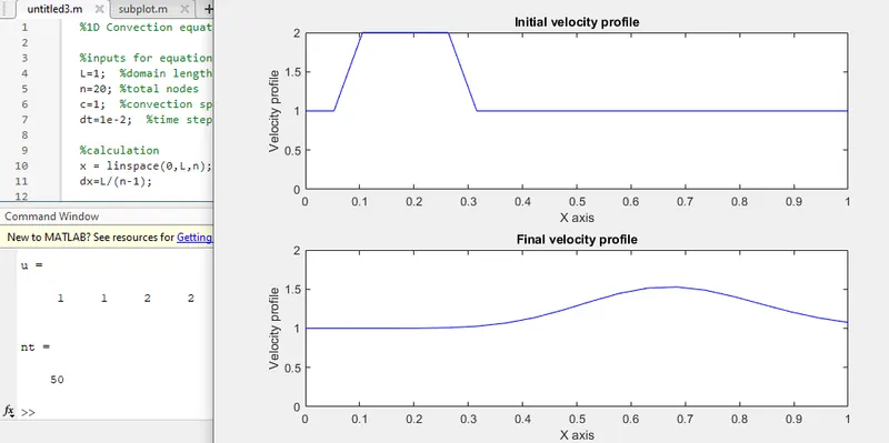
For total nodes 20, the accuracy of the graph is much less as seen below and at this point since the step is propogating right, the peak value of velocity is reducing drastically, as diffusion is dominating the behaviour.

Case 2 : 40 nodes

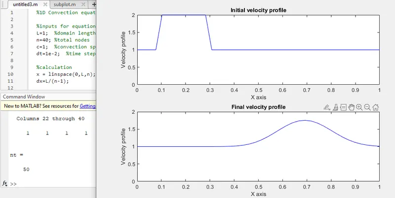
In case where total nodes are 40, the result is similar as previos one. though the effect of diffusion is slightly minimized.

Case 3 : 80 nodes

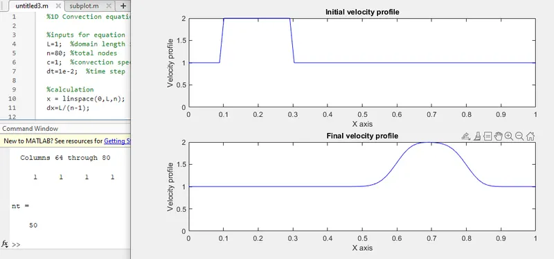
The solution here is quite smooth, as the diffusion is hardly affecting the movement of the square wave and the peak velocity is not dropped, however this is some curvature present at the both sharp corner of the step. This means that with increment in number of nodes, the solution tends to smooth out.

Case 4 : 160 nodes

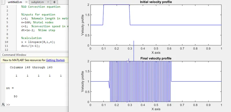
Here despite doubling the nodes from 80, the solution is unstable as there are oscillations is propogation and they eventually increse over time. This accounts the reverse behaviour as at some point, if the node(or grid) size is kept on increasing then the step shape is improved and so the output is smoothened, whilst, if nodes are increased beyond a certain limit, with same velocity of convection, it makes the approximation of the solution unstable and it might require a different scheme to be used.