Week 8 - Simulating Cyclone separator with Discrete Phase Modelling

Introduction to GUI based CFD using Ansys Fluent

Week 8 - Simulating Cyclone separator with Discrete Phase Modelling

Empirical models of cyclone separator:

1. Iozia and Leith Model

Iozia and Leith model is a modified version of is developed based on the force balance.
The model assumes that a particle carried by the vortex goes thru the influence of two forces, a]. centrifugal force and b]. flow resistance. The collection efficiency ηi of particle diameter
dp can be calculated from;

`η = 1 /(1 + ((dpc)/(dp))^beta`

Here dp is particle diameter in inlet and dpc is cut particle diameter of 50% efficiency.

2. Li and Wang Model

This model includes particle bounce or re-entrainment and turbulent diffusion at the cyclone wall. Its assumption is ;

a]. The radial particle velocity and the radial concentration profile are not constant for uncollected particles within the cyclone

3. Koch and Licht Model

Koch and Licht described particle motion in the entry and collection regions with the additional following assumptions;

a]. The tangential velocity of a particle is equal to the tangential velocity of the gas flow, i.e. there is no slip in the tangential direction between the particle and the gas

b]. The tangential velocity is related to the radius of cyclone by: `mu*R^n` = constant

4. Lapple Model

Lapple model was developed based on force balance without considering the flow resistance. Lapple assumed that a particle entering the cyclone is evenly distributed across the inlet opening. The particle that travels from inlet half width to thewall in the cyclone is collected with 50% efficiency.

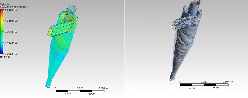
The following analysis of cyclone separator involves Discrete Phase Modelling technique (DPM), which is employed to represent solid particles in gas or liquid or liquid droplets/ bubbles in liquid medium. In DPM, two phases are considered, one is Continous phase (the fluid, here air, flowing thru the fluid volume) and second is Discrete phase that involves the small particles. The Discrete phase can exchange energy and momentum with the continous phase.

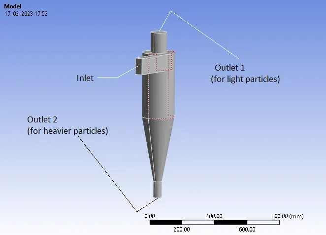
The geometry is loaded in Spaceclaim and an inlet plus two outlets are selected so as to create an interior fluid volume, as rest of the geometry is suppressed. Thereafter named selections are made.

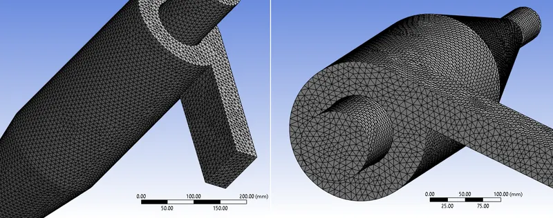
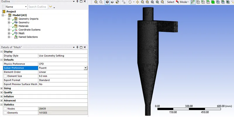
Secondly the entire geometry is discretized into small parts.

Fluent Setup;

Solver : Pressure Based

Type : Steady state

Gravity : Enabled, -9.81 `m/(s^2)`

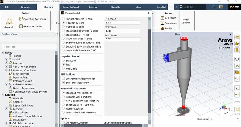
The viscous model is selected to RNG k-epsilon, with Standard wall functions and "Swirl Dominated flow".

With regards to the Discrete Phase modelling; it has two options.

a]. Coupled flow - The discrete phase (as small particles in present case) will influemce the continous phase (fluid flow).

b]. Uncoupled flow - The discrete phase will not have any interactions with the continous phase.

For this analysis, the Coupled flow is chosen as the particles' diameter is small so it will not have any significant variation, however selection of either of one depends on the size of the injected particles.

The DPM update interval is kept 10 (default) to track the particle behavior.

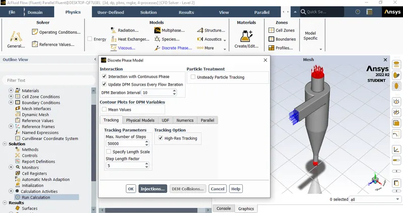
The maximum number of time steps are 50,000, which calculates a single particle trajectory. Beyond, this limit, the solver will stop tracking the trajectory of a particular particle in case if that particle goes on recirculating. In case of selecting "Specifying Length scale", the time step size will be calculated by dividing length scale by velocity of particle in discrete phase and in continous phase. If the value of length scale is less, then tracking the trajectory will be more accurate, with less time step size and larger Step length factor.

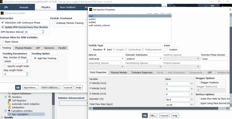
The injection type is set to inert and surface injection for anthracite coal particles thur inlet port. Subsequently, the velocity and diamater are set as required for analysis.

As there are ports present, the Boundary conditions are given as follows:-

Inlet:-	Velocity inlet and Reflect the discrete phase particle
Outlet 1:-	Pressure outlet and escape
Outlet 2:-	Pressure outlet and trap

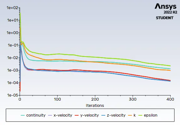
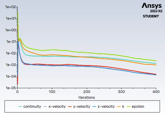
In the next stage, the Standard initialization is done via computing the values of inlet and the setup is ran for two different cases for 400 iterations with calculation of Separation Efficiency, which is given by;

Separator Efficiency = (Number of particles trapped)/(Number of particles tracked)

CASE 1 : Varying particle size and same velocity

Diameter`(mum)`	Velocity (m/s)	Particles Tracked	Particles Trapped	Particles escaped	Efficiency(%)
1	3	142	137	5	96
3	3	142	138	4	97
5	3	142	140	2	98

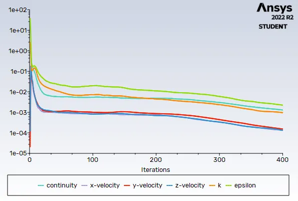
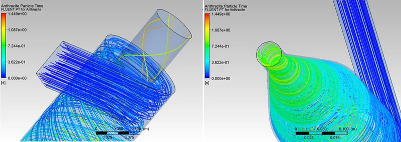
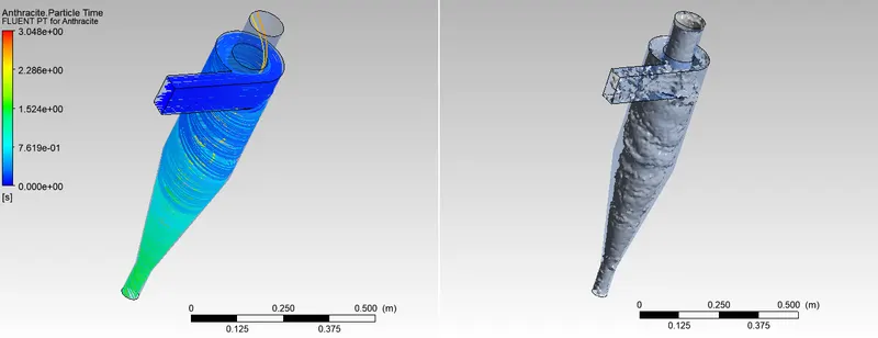
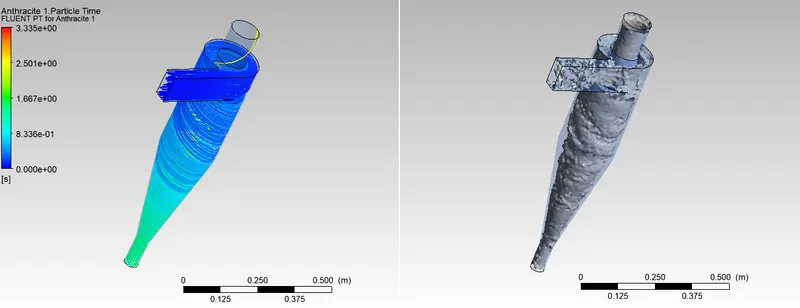
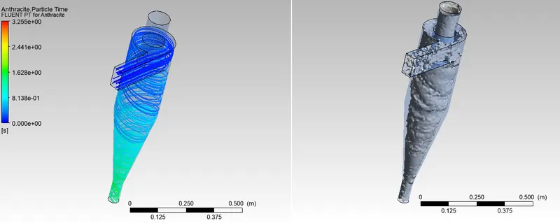
Residuals and contour plots of particle time and vortex strength:

d=1 micrometre and v=3m/s

d=3 micrometre and v=3m/s

d=5 micrometre and v=3m/s

CASE 2 : Varying velocity and same particle size

Diameter`(mum)`	Velocity (m/s)	Particles Tracked	Particles Trapped	Particles escaped	Efficiency(%)
5	1	142	136	6	95
5	3	142	140	2	98
5	4	142	135	7	95
5	5	142	127	15	87

Residuals and contours od particles' time, pressure variation, mass flow rate variation and voretex strength.

d=5 micrometre and v=1 m/s

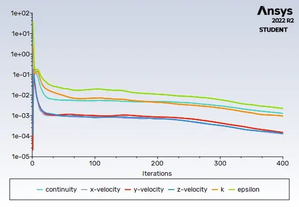
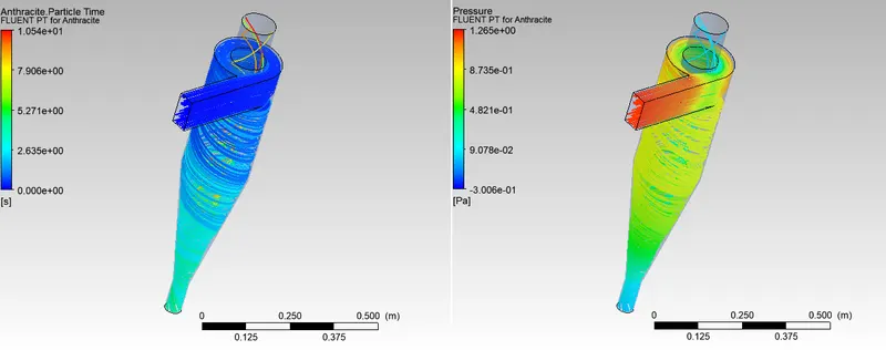
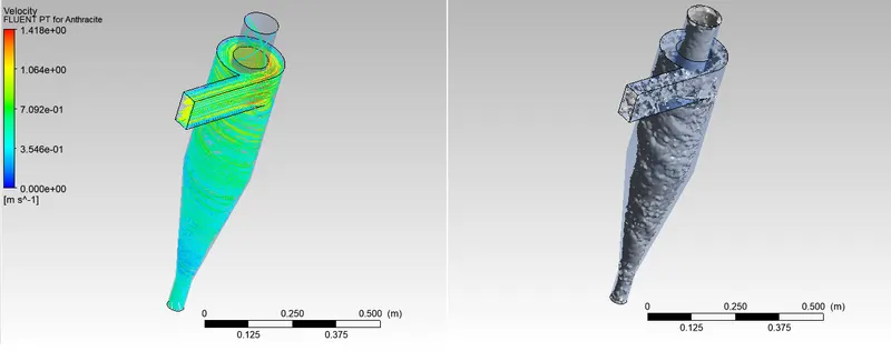d=5 micrometre and v=3m/s

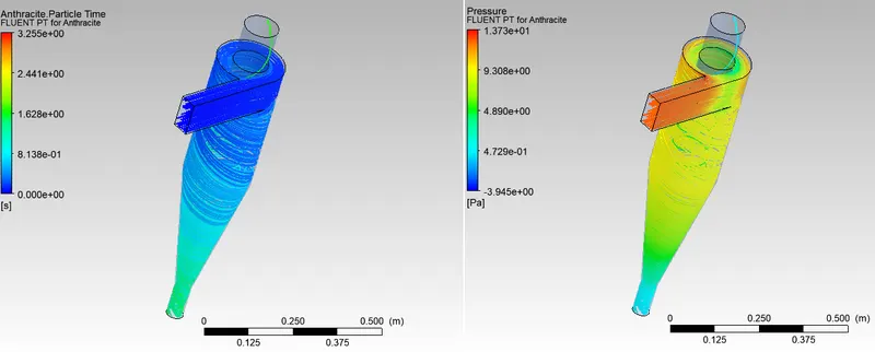
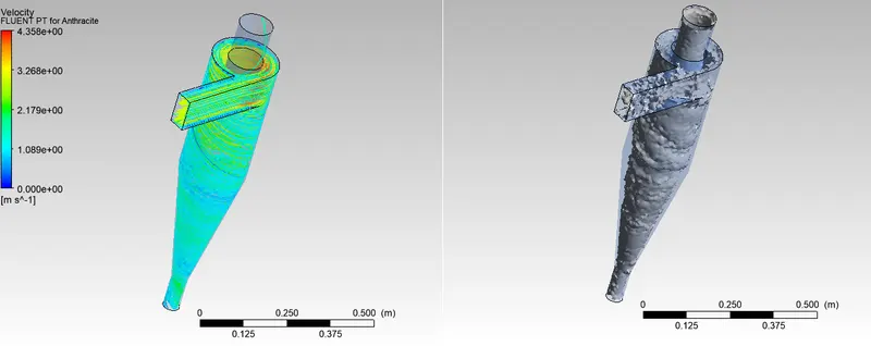
d=5 micrometre and v=5m/s

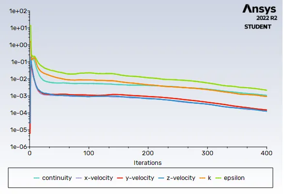
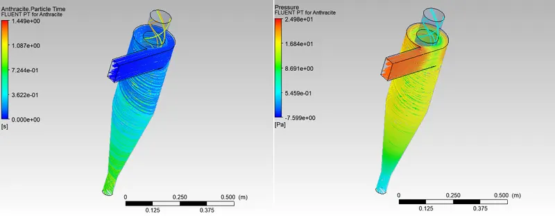
Conclusion

As seen from the table of case 1 and 2, as the diameter of anthracite particles increases, the efficiency of the cyclone separator also increases, whereas with the same particle size, as the flow velocity increases, a slight declination in the efficiency is obsereved.