Week 5: Prandtl Meyer Shock problem
Advanced Aerodynamic Simulations using Converge Studio
Week 5 Project :- Prandtl Meyer Shock problem
Shock-wave theory:
Shockwaves are pressure waves having large amplitude, that are created when the flow is faster than the speed of sound, i.e. with a velocity of more than 340 m/s or the Mach Number (M) greater than 1.
In the image shown below, the source is moving at a speed 'u' m/s which is less than the sound speed 'a'. After that, the velocity of object and the speed of sound in the regime are equal, hence the flow at the tip section of the object is under high compression at this stage, this case has M=1.
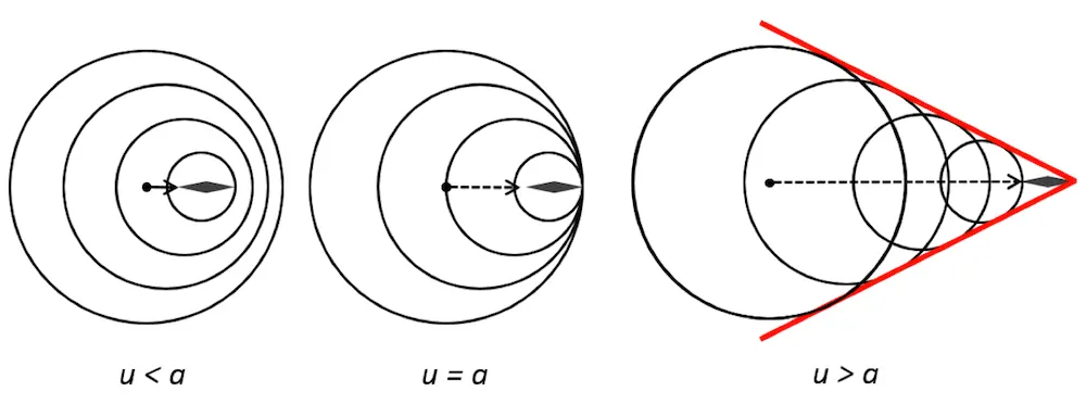
As soon as the the object's speed exceeds the speed of sound, this compression wave formed gets bursted, creating a jump in pressure and other thermodynamic properties. The mach waves, forming a mach cone, shown with red pattern in the third picture, gets narrowed as the speed of the moving object increases. While, in the supersonic flow, if the body surface turns away from the flow direction, an "Expansion fan" is formed at the corner. The pressure at the downstream reduces and the flow accelerates as it moves thru the expansion fan, and the flow here is 2-D isentropic.
Boundary conditions for simulating an expansion fan:
Inlet:
The inlet here has to be kept supersonic, the Dirichlet boundary condition is assigned, which means the fixed values, in magnitude, of all parameters is given.
Outlet:
Here the Neumann boundary condition is imposed, as a limitation in terms of partial derivative is given. Hence the value is put to Zero normal gradient, which means that all variables are set to a fixed value, and considering a variable is fully developed at the inflow region of the opening, so its variation with respect to space (`vecn`) is zero, i.e.`(dphi)/(dvecn)=0` .
Wall:
Since the flow here is at very high velocity, an assumption can be made the the flow can slip at the wall surface. It is assumed that at very high Reynolds Number, the ratio of frictional velocity to the free stream velocity, i.e. `(u)/(U)` is less than 0.01.
Adjacent faces:
At the faces, the planar assumption is made as the flow gradients along the z direction are negligible as compared to other two direction, required that the flow is taking place in x direction in x-y 2D plane.
Geometry setup and Pre-processing:
For the given project, the CAD model of the flow domain is loaded in the studio and since there are no errors in the geometry file, the scaling is done by factor of 0.001, following the similaritiy laws.
Nextly, the boundary flagging is done as per described above.
Solver Settings:
In the Time-Based type of Transient state simulation, the fluid is chosen as 'Air', as mixture of N2 and O2 of 0.77 and 0.23 percent.
Going with the case setup, the Redlich-Kwong equation is used as Equation of state as it is generally more accurate than the Ideal gas equation at temperatures above the critical temperatures, which is given as;
`p = ((R*T)/(V-b)) - ((a)/(sqrtT*V(V+b)))`,
where p is the Pressure
R is the Gas Constant
T is Temperature
V is Molar Volume (V/n)
a is a constant correction for attractive potential of molecules
b is a constant that corrects for volume
The Turbulent Prandtl number is a non-dimensional term defined as ratio between momentem eddy diffusivity and heat transfer eddy diffusivity. It is useful to solve heat transfer problem boundary layer flows. The summation of molecular and turbulent conductivity and diffusivity is taken into consideration when solving transport equations. With that, the turbulent Schmidt (Sc) and Prandtl number (Pr) are partially varying as presence of walls affect these values hence the default values taken near to 0.78 and 0.9 respectively. This default values is proved to be satisfactory for many reacting and non-reacting turbulent flows hence they can be used as some default approximations.
The case is set for full hydrodynamic and compressible flow and solver is preferred steady state solver. Initial minimum time step of 1e-7 and maximum time step of 1 with maximum convection CFL limit of 1. The lesser the CFL number's value is, the slow will be the simulation and more accurate will it be. In addition the convective flux scheme is set as FVM and the Density based solver is used. These particular values of Convection CFL, Diffusion and Mach CFL number is related to the stabilty of the solution which Converge uses as default.
With regards to the Boundary condition, all fixed values are provided with Inflow Boundary condition, with static pressure of 101000 Pa, velocity of 678 m/s with air as mixture of O2 and N2 being working fluid.
For the outflow, the Zero normal gradient is given, `n*nabla=0` as the fluid flows out of the domain.
In case of walls, instead of No-slip, the Slip condition is given, meaning that the flow being at very high speed is not viscous (inviscid), so at wall, the flow can slip, i.e. `v ≠ 0`.
For the faces, 2D planar assumption is made.
In the next stage the base grid size is kept 0.8 m, with total cell count of roughly 43000 cells. Here, the adaptive mesh refinement is employed, which monitors the curvature in temperature, i.e. `(del^2T)/(del^2x)`, lets say if the value of sub grid scale is 0.05, so if that curvature in flow gets more than the value 0.05, the mesh then gets refined automatically to accurately monitor the value of temperature at specific grid points. The base mesh is of 0.8 m, and with 2 levels of refinement, the grid will change as;
`Grid size = (base grid)/(2^(embed-layers)`
Hence the base grid will be 0.8 m, the second level will be 0.2 m.
The emphasis is not given on the selection of the viscous model, as there will not be any stress components produced because of inviscid flow, however, the default RNG k-epsilon is used.
The case is ran for two different velocities with base and refined mesh. After this the input files are exported to the case's setup folder and required executables along with license file are copied, and the case is analysed with 4 parallel processor in Cygwin. As the post processing of output files is done, the contours are viewed in Paraview and variation of parameters in Converge's line plot.
Post Processing:
CASE 1.a : v = 100m/s , mesh size = 0.8 and SGS = 0.05
Variation in velocity:
Variation in Mach number:
Variation in pressure:
Variation in temperature:
CASE 1.b : v = 678 m/s , mesh size = 0.8 and SGS = 0.05
Variation in velocity:
Variation in Mach Number:
Variation in Pressure:
Variation in Temperature:
CASE 2.a : v = 100 m/s , mesh size = 0.4 and SGS = 0.03
Variation in velocity:
Variation in Mach number:
Variation in pressure:
Variation in temperature:
CASE 2.b : v = 678 m/s , mesh size = 0.4 and SGS = 0.03
Variation in velocity:
Variation in Mach number:
Variation in pressure:
Variation in temperature:
Following is noted from the above graphs:
1. For Sub-grid scale 0.05, Mesh size = 0.8, Total cells = 43467
| 1. | Inlet Velocity (m/s) |
Outlet Velocity (m/s) |
Inlet Temperature (K) |
Outlet Temperature (K) |
Inlet Mach No. | Outlet Mach No. |
Inlet Static Pressure (Pa) |
Outlet Static Pressure (Pa) |
Inlet Density (kg/m⊃3;) |
Outlet Density (kg/m⊃3;) |
| a. | 100 | 380 | 286 |
171 |
0.29 |
1.44 | 101000 | 14524 | 1.225 |
0.287 |
| b. | 678 | 700 | 286 | 270 | 1.99 | 2.12 | 101000 | 82760 | 1.225 |
1.050 |
2. For Sub-grid scale 0.03, Mesh size = 0.4, Total cells = 245241
| 2. | Inlet Velocity (m/s) |
Outlet Velocity (m/s) |
Inlet Temperature (K) | Outlet Temperature (K) | Inlet Mach No. | Outlet Mach No. |
Inlet Static Pressure (Pa) |
Outlet Static Pressure (Pa) |
Inlet Density (kg/m⊃3;) |
Outlet Density (kg/m⊃3;) |
| a. | 100 | 375 | 286 |
172 |
0.29 | 1.41 | 101000 | 14567 | 1.225 | 0.29 |
| b. | 678 | 696 | 286 |
271 |
1.99 | 2.12 | 101000 | 83253 | 1.225 | 1.059 |
Conclusion:
As seen from the graph where the inflow velocity is 100 m/s, with M~0.3, nearly compressible, the flow when it turns away from the surface, is seemed to be expanded with a gradual rise in velocity at the downstream region, whereas, a slow declination is observed in the plots of static pressure, temperature and density. Here, the stagnation pressure and temperature remains constant at upstream and downstream.
With regards to the plots with incoming velocity of 678 m/s, a sharp expansion wave is generated, creating sudden changes in thermodynamic properties. In the variation of velocity and Mach number, an abrupt change is seen causing an increment in the outlet parameters. Similarly, a jump is seen where the temperature and static pressure, along with the density, falls.
Considering the case where the sub-grid scale is 0.05, the curvature in temperature is monitered at only a specific region, i.e. where fan is generated, which implies that in the near zones the variation in `(del^2T)/(delx^2)` is less than 0.05 and it does not exceed the given value, however, for the second case, with SGS of 0.03, the area of expansion fan along with the near about zones are monitered where the curvature in temperature surpasses the value of 0.05 as well as 0.03 too. At these zones, the mesh is refined indicating that properties of air molecules is varying and amount of heat changes with interaction in surrounding.