Week 2 - Flow over a Cylinder.
Introduction to GUI based CFD using Ansys Fluent
Week - 2 : Flow over a Cylinder
Objective : To simulate the flow over a cylinder and visualize the effect of vortex shedding at different Reynolds Number.
To begin with, a 2D geometry is created in Spaceclaim with a cylinder, here as cross sectional view of circle with diameter 2m, with certain distance from inlet and outlet. The sketched geometry is pulled to make a domain with a cylinder, and nextly the faces of the domain field are named as inlet, outlet, and walls with symmetry boundary condition.
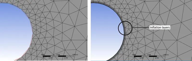
For the meshing, instead of accounting a default mesh, a triangular mesh is constructed with element size 0.25, which is very fine. Secondly, the circular cyliner is not perfectly circle so, sizing is done with 36 nodes at 10 degrees to make the curvature more smoother. Now, in order to capture the surface effects, Inflation layers are added around circumference, with layer thickness of 0.006m and a Growth rate of 1.2, which implies the gradual increment of thickness as moving away from the primary inflation layer.
Once the mesh is done, physical conditions are setup in Fluent.
Part 1 : Simulate the flow with the steady and unsteady case and calculate the Strouhal Number for Re= 100.
1.a) Steady case at Re = 100
Here, considering the Re = 100, for Laminar regime, following fluid and Boundary conditions are kept for setup.
| Inlet : Velocity inlet | 1 m/s |
| Outlet : Pressure outlet | 0 Pa |
| Wall : No slip condition | 0 velocity at surface |
| Density (`rho`): | `1 (kg)/m^3` |
| Dynamic viscosity (`mu`): | `0.025 (Ns)/(m^2)` |
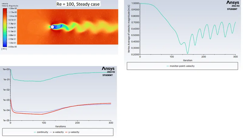
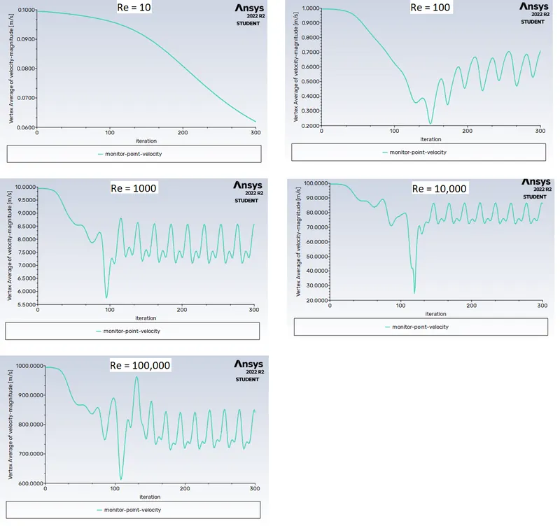
For monitering the flow behaviour past a cylinder, a monitoring point is created at centre. With Hydrid initialization for giving out initial velocities, "Pressure based Solver" is chosen as the problem falls in nearly incompressible region. The solver solves the corrected values of pressure and velocity for convergence, Continuity equation, x-momentum, y-momentum and z-momentum equation.
The plots are made by defining the reports for iterations of residuals, velocity contours and Vertex average report with the created reference point. The calculation is run for 300 iterations, with convergence check disabled for viewing the results.
1.b) Unsteady case at Re = 100
For the transient case, as the parameters are time dependent, there is a specific frequency at with the vortices are shedding, this frequency is directly proportional to the Strouhal Number (Sr), indicates the oscillations in a flow.
`Sr = (f.d)/(v)`
where f = frequency of oscillations, Hz.
d = length of object, m.
v = fluid velocity, m/s.
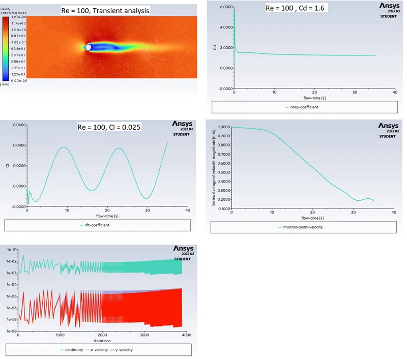
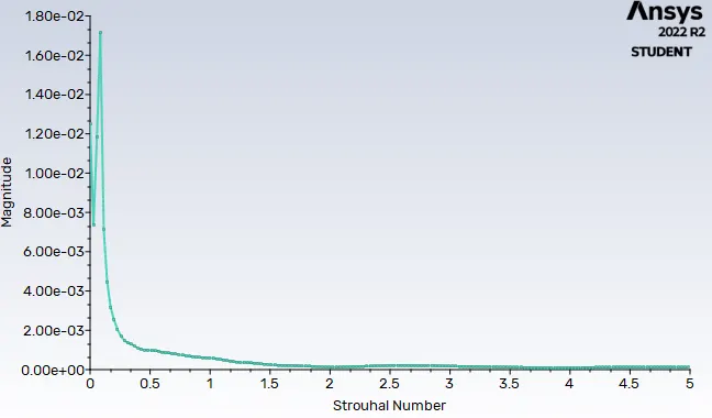
The transient simulation is run for 450 iterations with a step size of 0.1. For plotting the Strouhal number, the lift coefficient file (oscillations) is taken for input, and the data will be converted to frequency by FFT (Fast Fourier Transform).
The Strouhal Number for the unsteady case is around 0.170.
Part 2 : Steady simulation for observing variations in lift and drag coefficients at different Re.
The cases are ran for Reynolds Number 10, 100, 1000, 10000 and 100000. The dynamic viscosity of the fluid is kept constant and velocity is varied for each case.
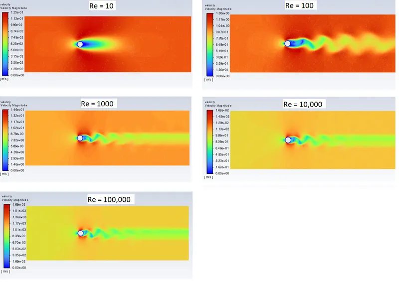
Plots of velocity contour at different Re:
Plots of vertex average magnitude at different Re:
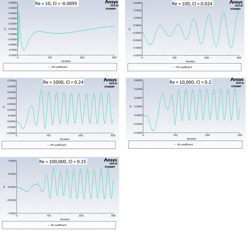
Plots of Lift coefficient vs. iterations at different Re:
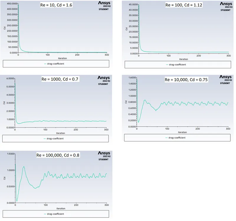
Plots of Drag coefficient vs. iterations at different Re:
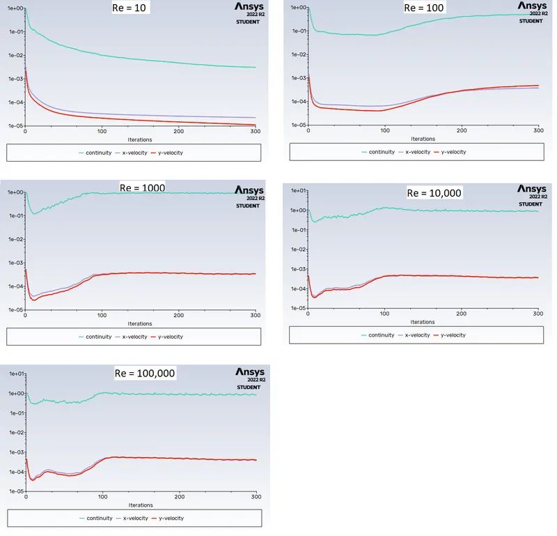
Plots of residual convergence at different Re:
Conclusion :
The following is noted from the plots;
| Re | Cl | Cd |
| 10 | -0.0095 | 1.6 |
| 100 | 0.024 | 1.12 |
| 1000 | 0.24 | 0.7 |
| 10000 | 0.2 | 0.75 |
| 100000 | 0.15 | 0.8 |
At Re 10, the flow when separates, the phenomena is symmterical. As the flow approaches, when Re = 100, a vortex pattern is visible at aft of cylinder surface, so vortices are shed from Higher and lower pressure zones of the cylinder. Until this point, the drag coefficient is not fluctuating highly, from the laminar vortex shedding there is a transition to turbulent wakes, from Re 1000 onwards.
The lift produced is varying largely, and the Cd is approximately in the range of 0.7-0.8 from `10^3 < Re < 10^5`[1]. Additionally at large values of Re, the turbulent boundary layer gets separated as well, with a subtle decline in lift coefficient. In case, if the flow converges then there will not nbe any intermittent fluctuations in plots of Cl and Cd, or at some point the pattern of oscillations will keep repeating after a certain point in iteration, however for smooth capturing of flow field, the results will also depend on grid size and number of iterations. Furthermore, with increase in Re, the Strouhal number will continue to rise as of more oscillations, and so values of Cl and Cd will swing dramatically [2].
References
[2] https://www.sciencedirect.com/science/article/pii/S0307904X08000243