Week 3: Flow over a backward facing step

Week 3 :- Flow over a backward facing step

Pre-processing:

For this challenge, the CAD model of '.stl' format of the backward facing step is loaded in the Converge Studio and is scaled by a factor of 0.001.

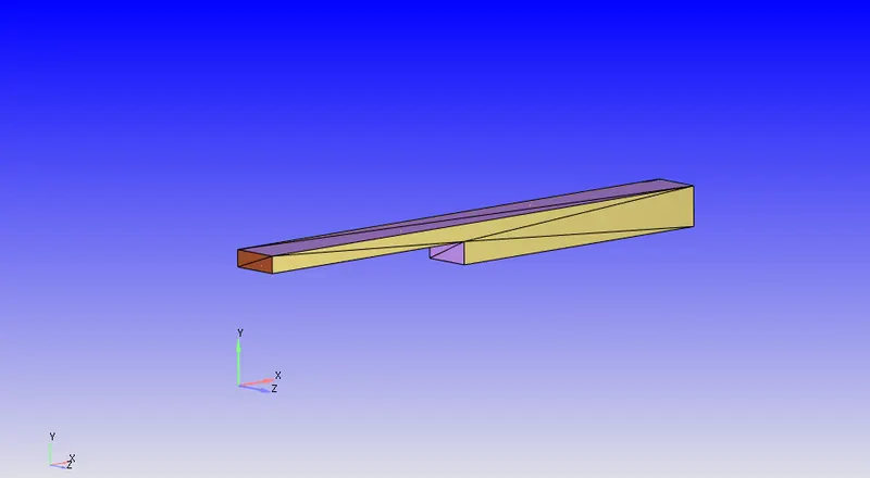
In the nexy stage, multiple boundaries are created. The boundaries are assigned as,

Front and back walls :- inlet and outlet

Adjacent walls :- 2 dimensional walls

Upper surface and the lower surface :- walls

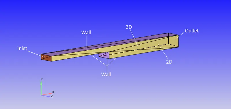
After the geometry setup is done the case setup is started.

Solver settings:

In the Time-Based type of simulation, the material is chosen as 'Air', as mixture of N2 and O2 of 0.77 and 0.23 percent.

The Turbulent Prandtl number is a non-dimensional term defined as ratio between momentem eddy diffusivity and heat transfer eddy diffusivity. It is useful to solve heat transfer problem boundary layer flows. The summation of molecular and turbulent conductivity and diffusivity is taken into consideration when solving transport equations. With that, the turbulent Schmidt (Sc) and Prandtl number (Pr) are partially varying as presence of walls affect these values hence the default values taken near to 0.78 and 0.9 respectively.

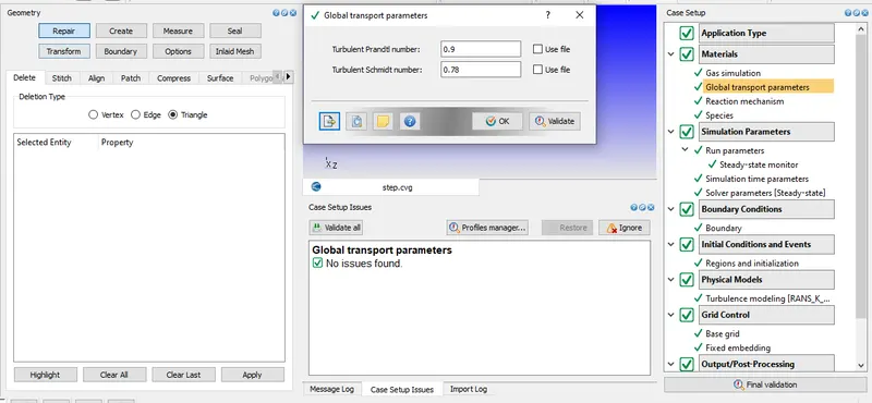
This default values is proved to be satisfactory for many reacting and non-reacting turbulent flows hence they can be used as some default approximations.

The case is set for full hydrodynamic and compressible flow and solver is preferred steady state solver.

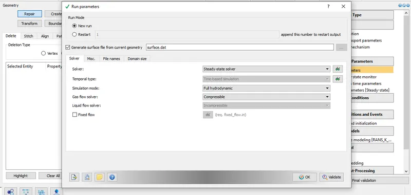
The end time for case is set to 8000 Cycles with initial minimum time step of 1e-6 and maximum time step of 1 with maximum convection CFL limit of 0.5. The lesser the CFL number's value is, the slow will be the simulation and more accurate will it be. In addition the convective flux scheme is set as FVM and the Density based solver is used. These particular values of Convection CFL, Diffusion and Mach CFL number is related to the stabilty of the solution which Converge uses as default.

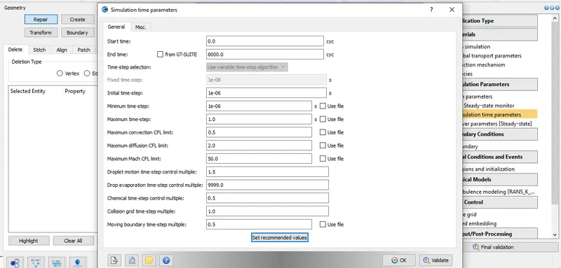
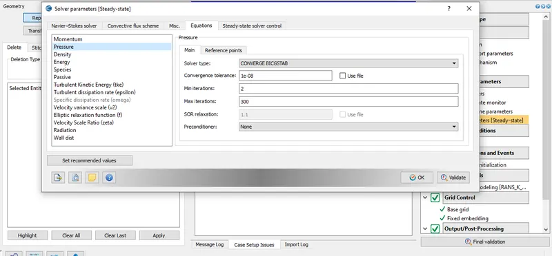
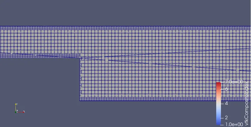
Along the X, Y and Z Direction the cell size is kept 0.001 meters with the total cell count of 100462. As those Governing equations are solved at each cell and they are PDE, however while solving those terms in the PDE are converted to algebraic form for making iterations, so while using the Pressure Preconditioner as 'None', solution is not that affected.

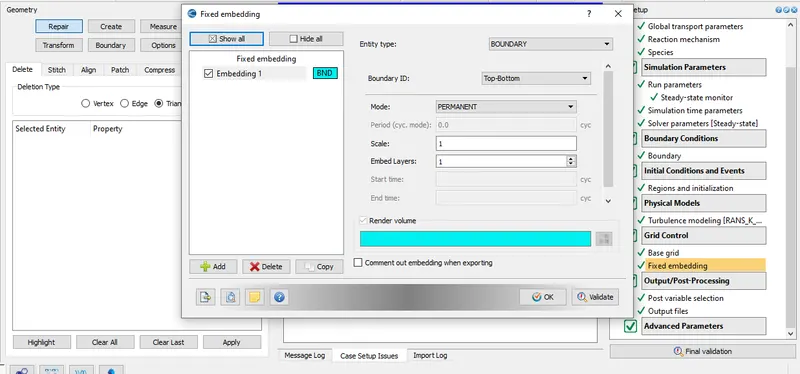
Secondly for embedding boundary type fixed embedding is provided with embed layers of 1-2 which captures the fine grid at some specific locations of the geometry. This is similar to the mesh refinement as boundaries as was done in Ansys Fluent.

In case of Viscous model selection, in the standard k-Epsilon model, the eddy viscosity is determined by single turbulent length scale, however in reality all scales of motion contribute to turbulent diffusion so is this modified equation of Renormalised Group, (RNG k-epsilon) it accounts for different scales through changes in the production term.

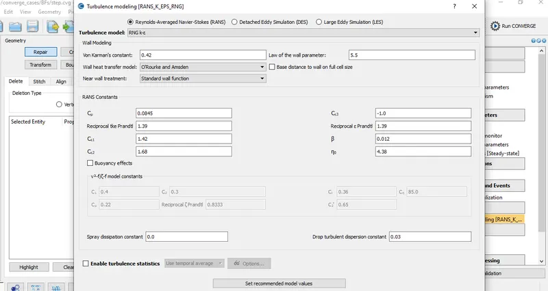
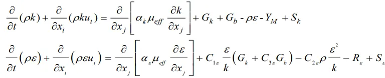
In above equations of RNG k-eplison model, the Gk is the term representing the formation of Turbulent Kinetic energy thru flow's mean velocity gradients.

With regards to the boundary conditions the inlet boundary condition is given to inflow with the Pressure Inlet of 110325 pascals and the outlet pressure of one atmosphere which is 1 atm, i.e., 101325 pascals. Hence from this it is concluded that the inflow velocity is around 120 m/s which is nearly compressible flow with Mach number, M = 0.3, the upper and bottom wall are given the wall boundary conditions of no-slip wall at surface the front and back is given at 2D boundary condition.

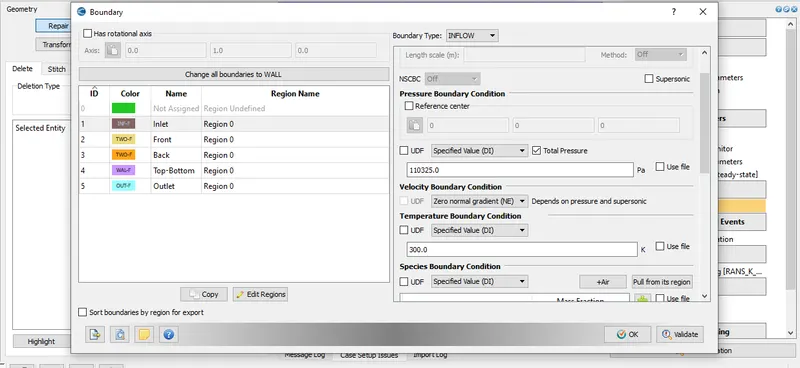
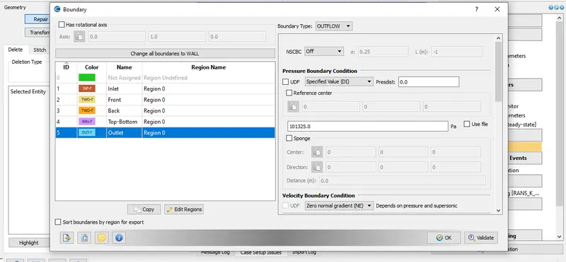
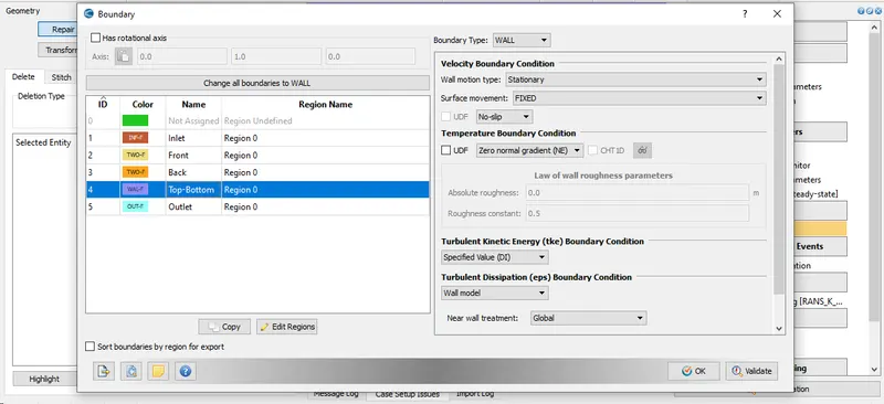
After putting the required executables and license. lic file in the setup folder, the cases are ran in the Cwgwin with four parallel processors with total of 8000 cycles and the output files are printed at every 200 intervals.

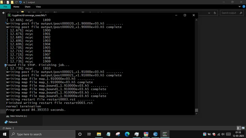
Now in order to view the post processed files in the Paraview the output printed files are converted in the suitable VTK format in the Converge Post processor.

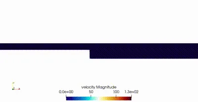
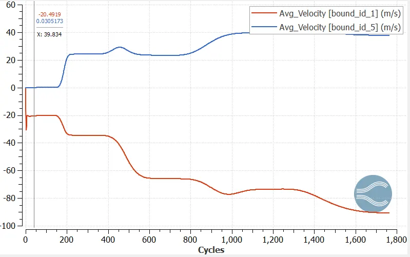
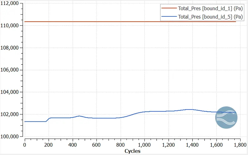
Apart from it the line plots the variation in the mass flow rate at Inlet and Outlet boundaries the variation velocity and total pressure is also plotted. In ParaView the contours for velocity, pressure and density are captured for three different grid sizes and there after the vector plot is formed showing the recirculation zone at the wall.

The case is ran for 3 different cases with mesh size and total cell count of:

Cases	Cell Size (metres)	Total cells (approx.)
1.	0.001	100462
2.	0.0009	137807
3.	0.00075	238131

Plots and contours:

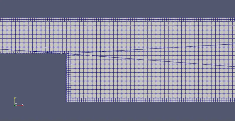
For Case 1: mesh for dx=dy=dz= 0.001 m.

Mesh size

Variation in Velocity

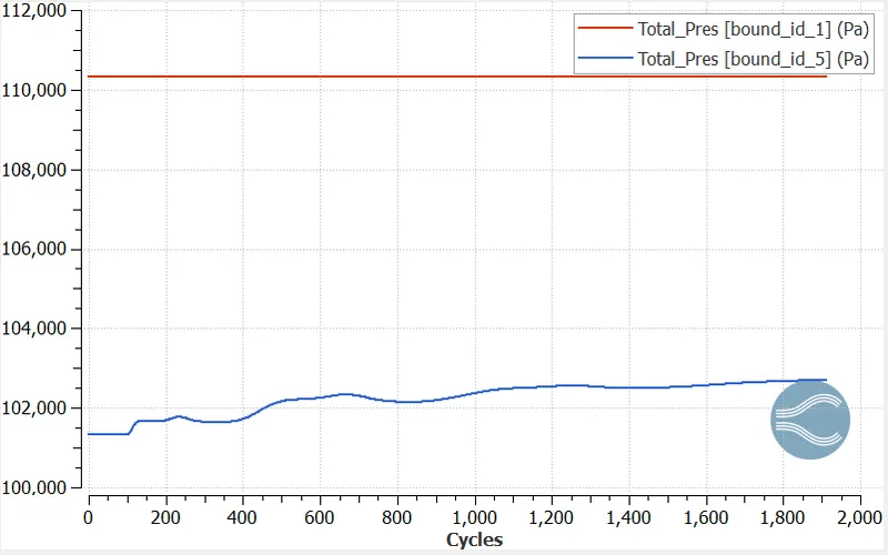
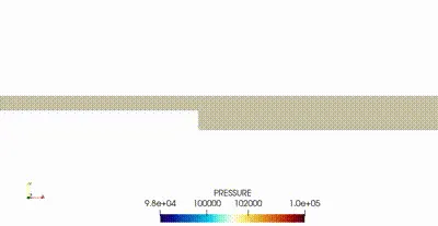
Variation in Pressure

Variation in Mass flow rate

For Case 2: mesh for dx=dy=dz= 0.0009 m.

Mesh size

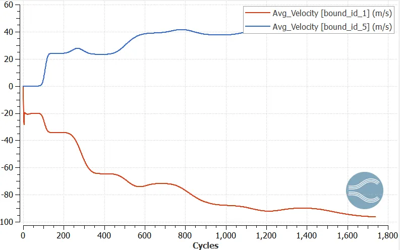
Variation in Velocity

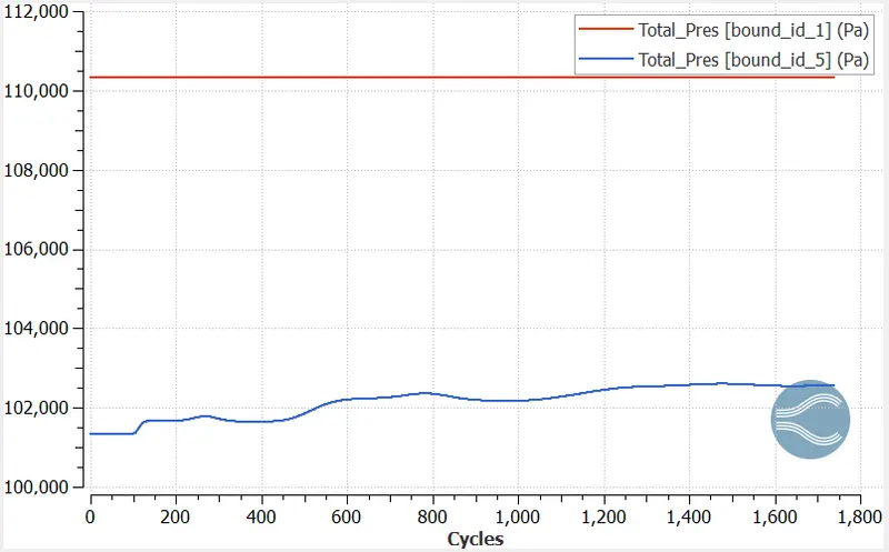
Variation in Pressure

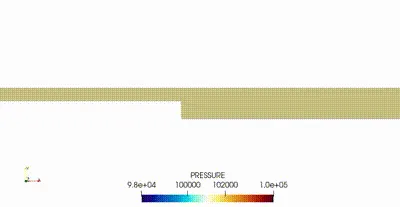
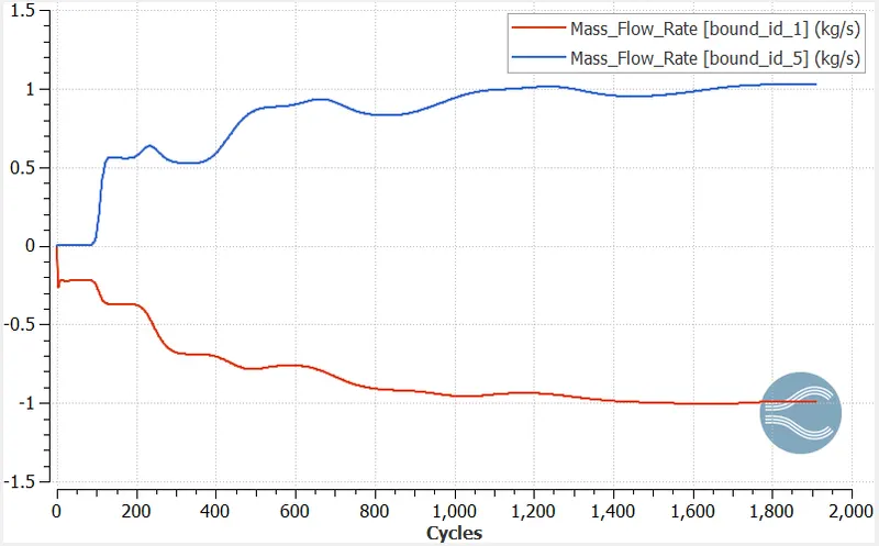
Variation in Mass flow rate

For Case 3: mesh for dx=dy=dz= 0.00075 m.

Mesh size

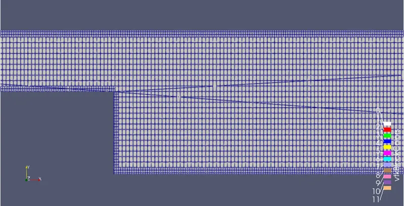
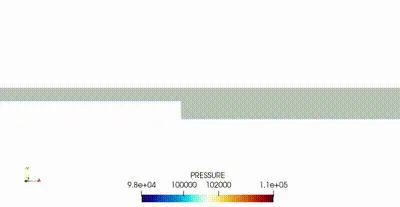
Variation in Velocity

Variation in Pressure

Variation in Mass flow rate

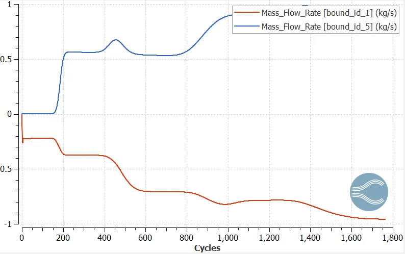
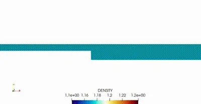
From the above plots, following is noted:

Sr.No.	Mesh size	Cells	Inlet Pressure (Pa)	Outlet Pressure (Pa)	Inlet velocity (m/s)	Outlet velocity (m/s)	Inlet Mass flow rate (kg/s)	Outlet Mass flow rate (kg/s)
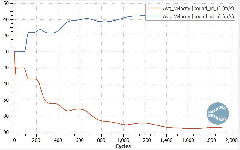
1.	0.001	100462	110325	102692	94	46	1	1.02
2.	0.0009	137807	110325	102563	96	44	1.01	0.96
3.	0.00075	238131	110325	102176	90	37	0.95	0.85

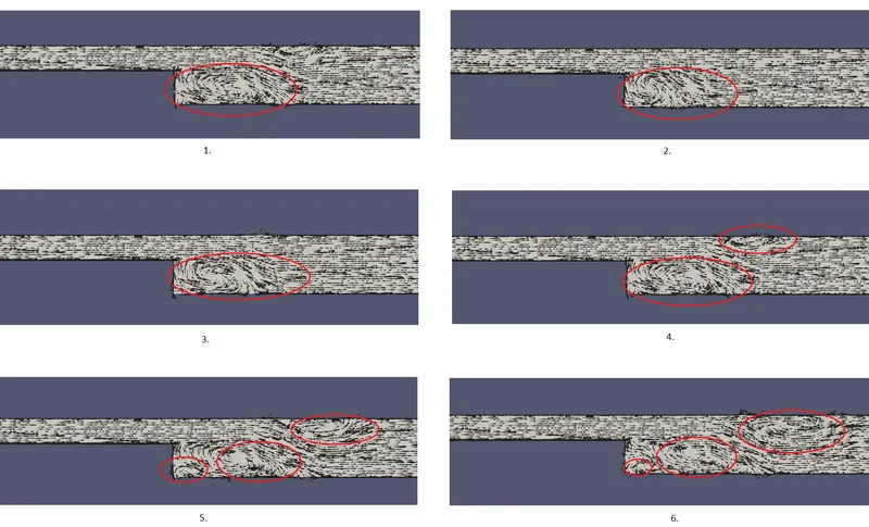
Visualization of Recirculation zone for 0.00075 metre grid setup:

Conclusion:

For the given mesh sizes, the convergence rate varies as the case with very fine mesh takes longer to converge the residuals and it requires more iterations.

From the values given in the table, it is clear that the outlet velocity is lesser than the input one, as of the flow velocity or say the velocity gradients are reduced with increase in pressure gradients (`(delp)/(delx)>0 and (delv)/(delx)<0`). This happens as while the flow comes from inlet, as shown in the picture containing velocty vectors, it is attached at the surface but since there is no surface after a certain distance, the flow starts to separate, and in that swirling region, the pressure is less, and as its a cyclic process, the bigger vortex slowly gets converted into the smaller vortices and so on. The accurate prediction of these swirling pattern also depends on the correct selection of the viscous model.

Secondly, after the stepped region, there is no surface present which can drive the flow forward with certain velocity, as an aftermath of this the air particles continues to roam in the fluid domain with unsteady and irregular motion. This visualization depends on the quality of the mesh created. A very high quality mesh captures the phenomena precicely and thereby predicting near correct values of pressure, velocity anf mass flow rate (averaged) from cells. As seen from the tabular values, the velocity and mass flow rate values differs in each case with variation in cell size, hence from the present given amongst three cases, the results of case three with smallest mesh size are more reliable.