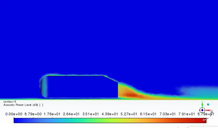
Week 11- Broadband Noise modelling over Ahmed body
Week 11 - Broadband Noise Modelling over an Ahmed Body
The Ahmed body is a car model, that was proposed in 1984 by Ahmed et al., and it serves as a benchmark to compute external flow analysis.
The Ahmed body creates the essential elements of the flow pattern surrounding an automobile, such as flow separation and wake production at the back, relative uniform air flow around the center section, and flow impingementation and displacement near the nose.
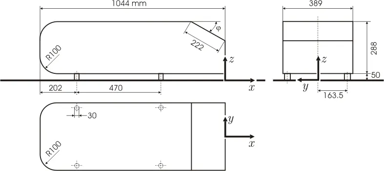
The model of the Ahmed body is imported to Spaceclaim.
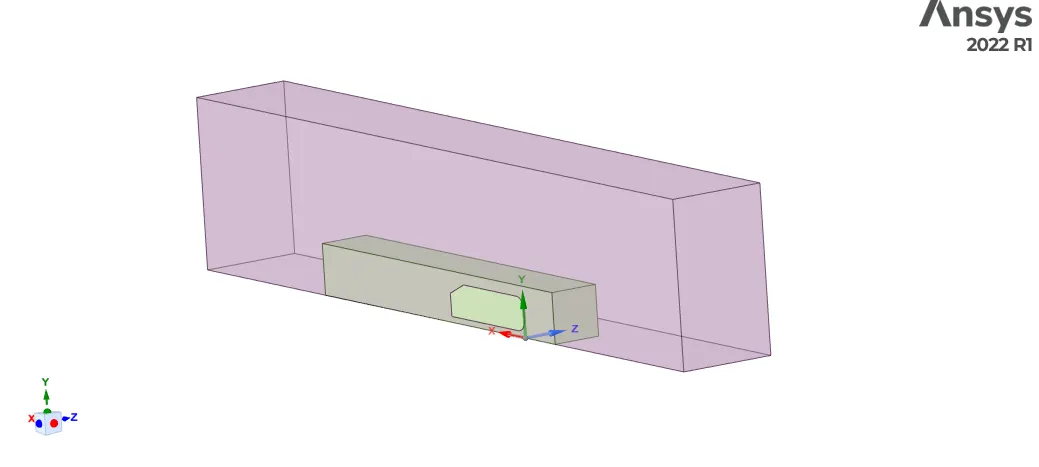
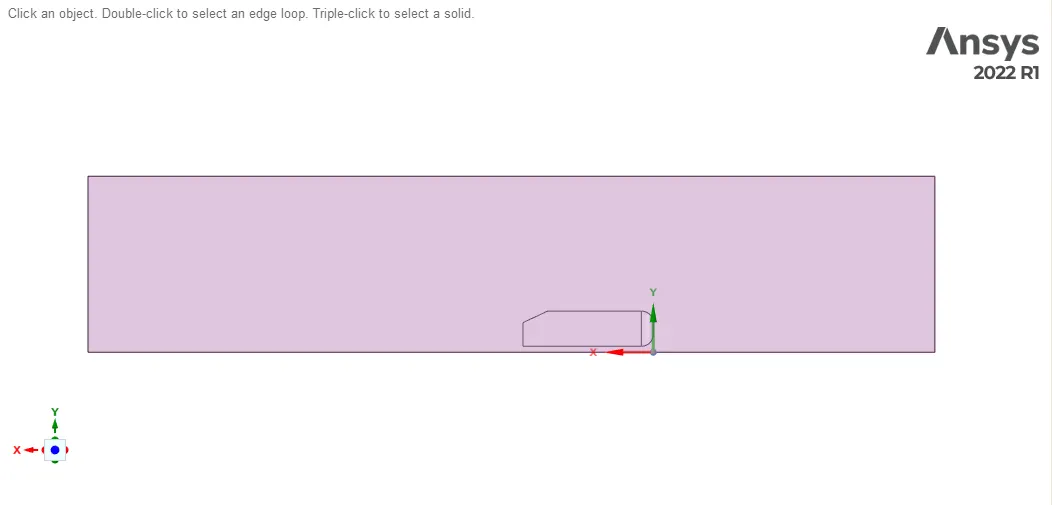
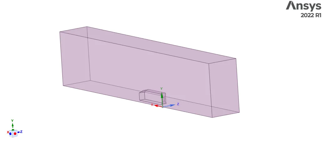
The model consist of a fluid domain with a small enclosure in it, and where the car object is subtracted from the whole domain so that the flow does not take place in it.
As the flow will take place over the body, to capture the boundary layer, prism layers need to be provided and few additional layers are provided on the road surface.
Mesh:
The model is imported to Mesh.
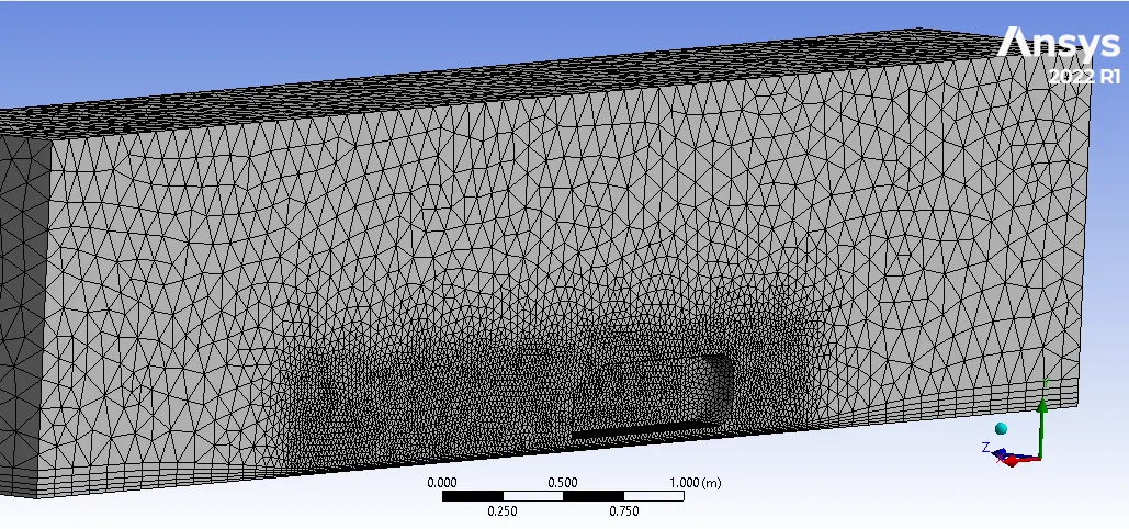
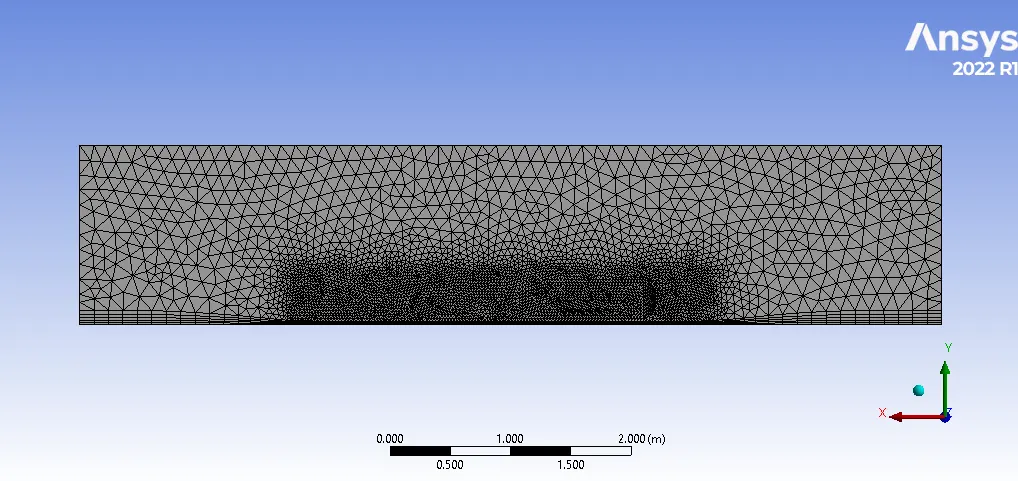
The global element size is kept 0.12m, the in enclosure sizing is kept 0.025m so as to get refined mesh.
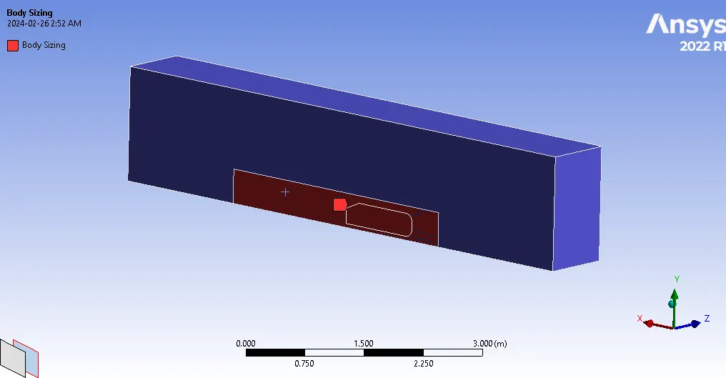
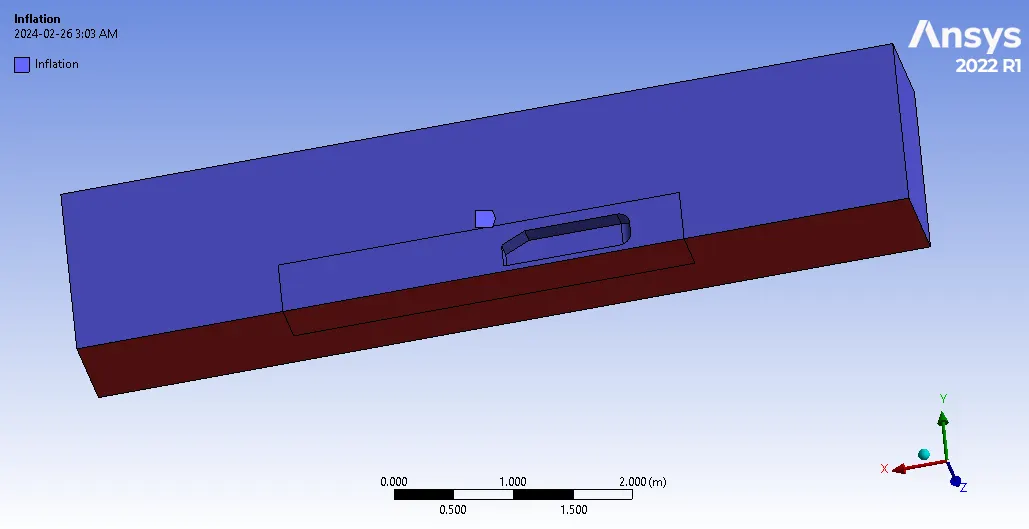
Five Inflation layers are added on road surface with smooth transition and the for the car, the first layer height is calculated based on following flow conditions.
| y+ | = 1 |
| Free stream velocity | = 31 m/s |
| Air Density | = 1.225 `(kg)/m^3` |
| Dynamic Viscosity | = 1.8e-05 kg/m |
| Characteristic length | = 1.09 m |
| Reynolds Number | = 2.2e06 |
| First cell height | = 1e-05 m |
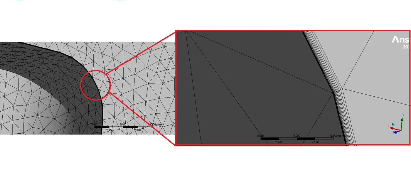
20 Prism layers provided on the car surface:
Solver Settings:
The solver is set to Pressure Based as it is low velocity flow.
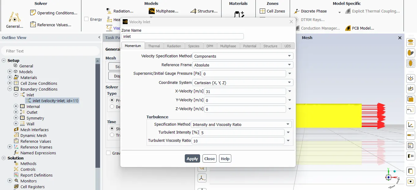
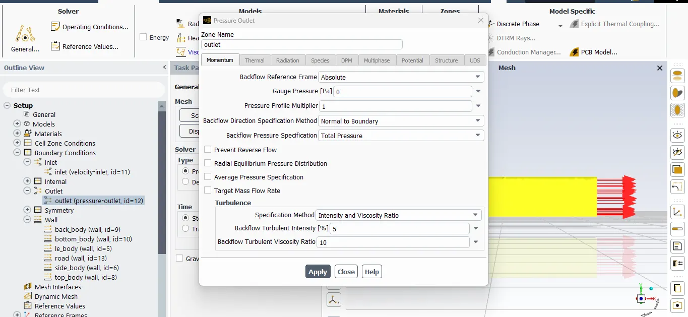
The inlet velocity is 31 m/s in X direction and Outlet pressure is 0 Pa.
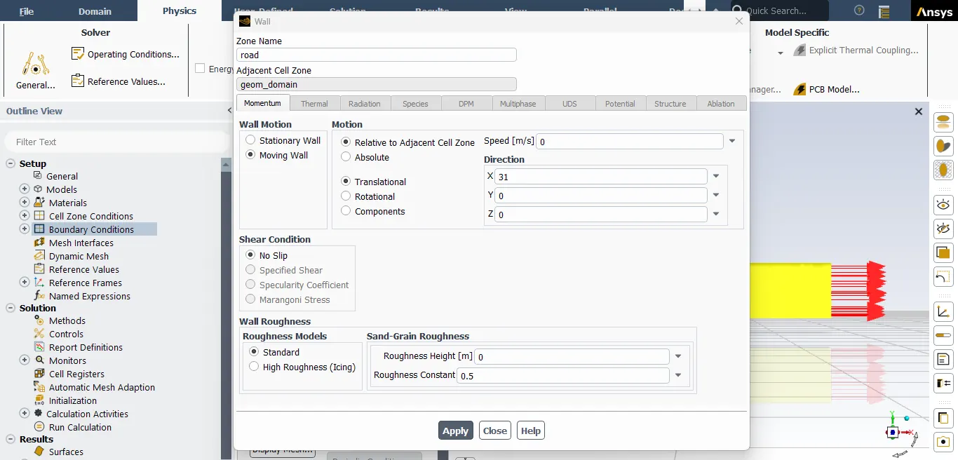
The Road surface is given Moving wall boundary condition with same velocity as 31 m/s.
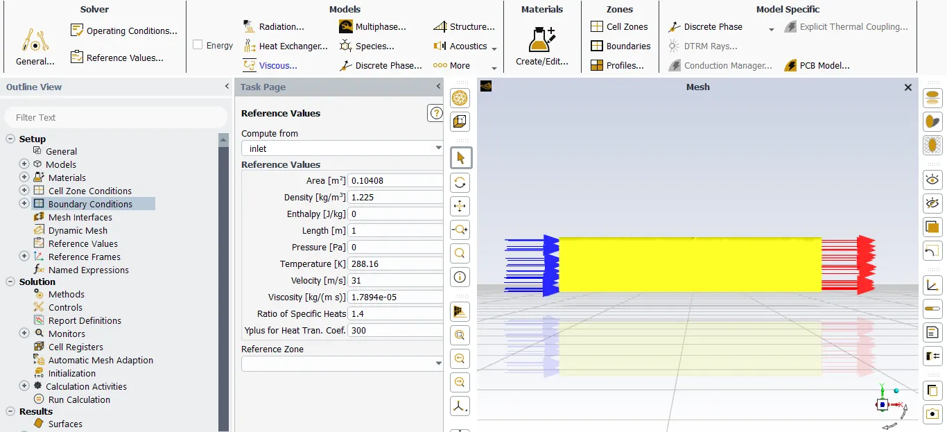
Reference values are to be calculated fom the inlet with frontal area of 0.10408 `m^2`.
The k-epsilon Realizable with Enhanced wall treatment is considered for the viscous model.
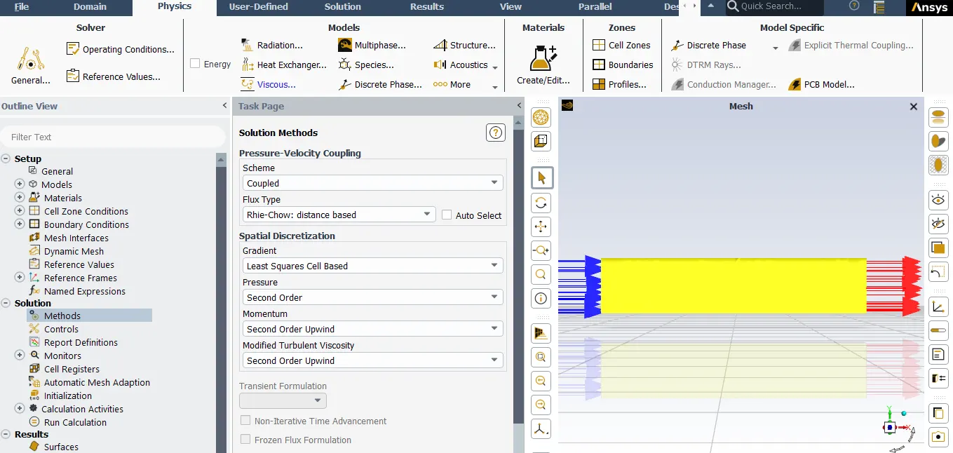
In the solution, the Pressure Velocity scheme is kept coupled.
Spatial Discretization which stores the discrete vales of scalar variables at cell centres is kept to Second order upwind for Momentum and Modified Turbulent Viscosity.
With standard initialization, the initial values are computed from inlet.
Plots and Contours:
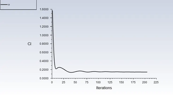
1. Variation in Lift coefficient:
The average Cl is around 0.144.
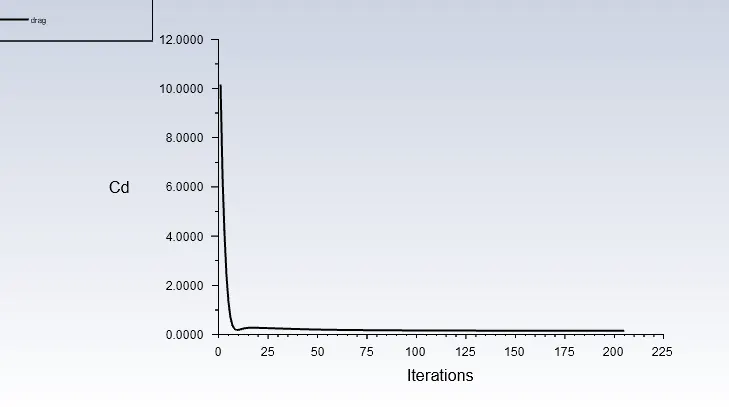
2. Variation in Drag coefficient:
The average Cd is around 0.154.
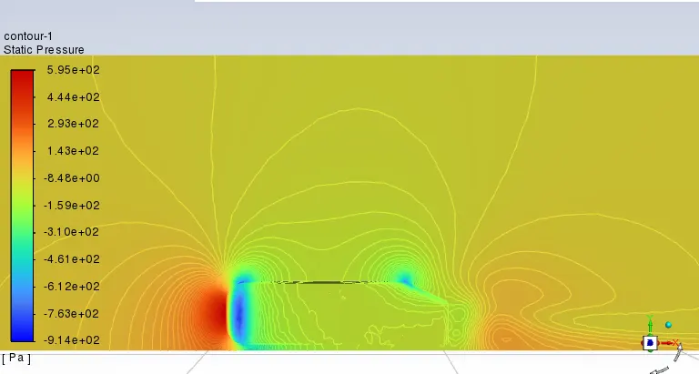
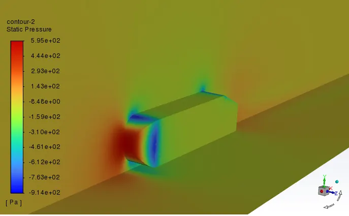
3. Contour of Static pressure:
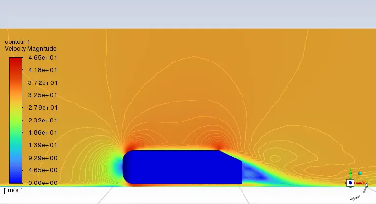
4. Contour of Velocity:
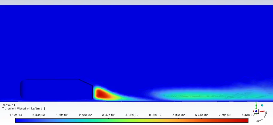
5. Contour of Turbulent Viscosity:
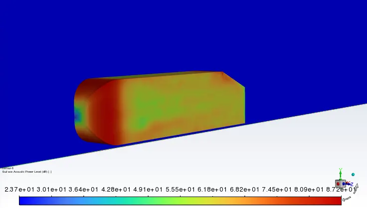
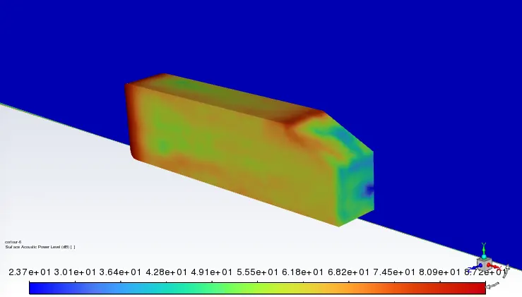
6. Contour of Surface acoustic power level:
7. Contour of Noise Level Disturbance:
The image below depicts the noise generation regions based on the setup, here the boundary layer and the wake formed are primary contributors to noise development.