Week 1: Channel flow simulation using CONVERGE CFD

Week 1 :- Channel flow simulation using CONVERGE CFD

Geometry setup and preprocessing:

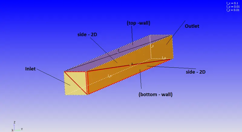
For the case, in order to simulate a simple airflow inside a rectangular closed passage, a duct is created with width and height of 0.1 metre and length of 0.1 metre, with normal `vecn` pointing in inner direction.

Solver Settings:

Thereafter, the different boundary ID is given to all 6 faces.

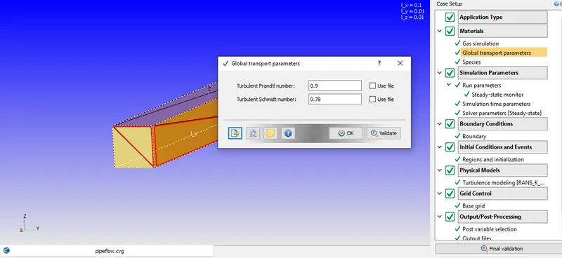
In the case setup, the fluid is set to 'Air' as mixture of N2 and O2 of 0.77 and 0.23 percent.

The Turbulent Prandtl number is a non-dimensional term defined as ratio between momentem eddy diffusivity and heat transfer eddy diffusivity. It is useful to solve heat transfer problem boundary layer flows. The summation of molecular and turbulent conductivity and diffusivity is taken into consideration when solving transport equations. With that, the turbulent Schmidt (Sc) and Prandtl number (Pr) are partially varying as presence of walls affect these values hence the default values taken near to 0.78 and 0.9 respectively.

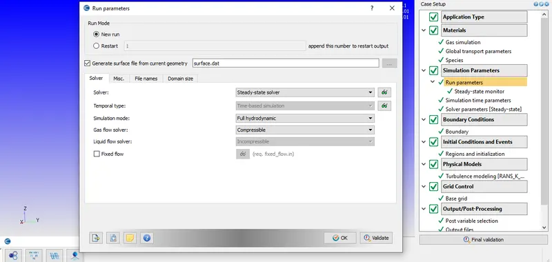
The case is set for full hydrodynamic and compressible flow and solver is preferred steady state solver.

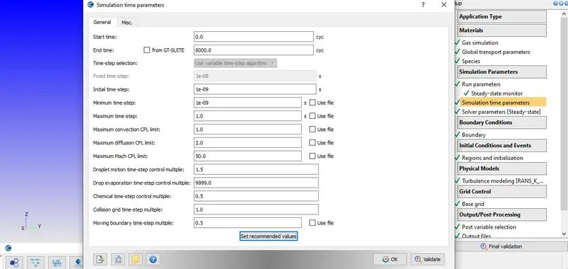
With regards to the simulation time parameters, the end time for case is set to 8000 Cycles with initial minimum time step of 1e-9 and maximum time step of 1 with maximum convection CFL limit of 1. The lesser the CFL number's value is, the slow will be the simulation and more accurate will it be. In addition the convective flux scheme is set as FVM and the Density based solver is used. These particular values of Convection CFL, Diffusion and Mach CFL number is related to the stabilty of the solution which Converge uses as default.

The solution scheme is set to PISO which is "Pressure Implicit with Splitting of Operator". The PISO algorithm with multiple time steps provides more stable solution, with lower time steps.

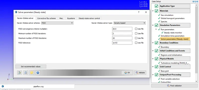
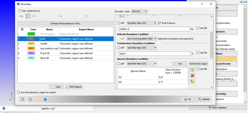
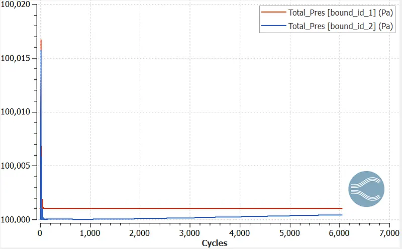
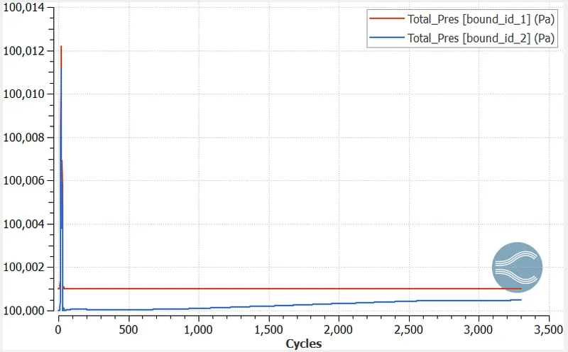
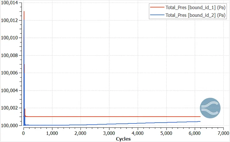
Nextly, the Inlet boundary condition is given as Pressure Inflow, with Inlet pressure of 100001 Pa and Outlet pressure of 100000 Pa. This pressure difference here drives the flow. The walls are set to No-Slip condition as the velocity at the surface is zero.

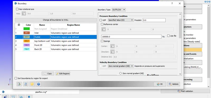
The left and right adjacent walls are given the 2-D symmetry conditions.

As the flow is viscous, the viscous model is selected to "RNG k-epsilon".

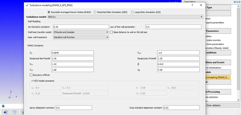
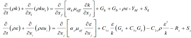
In the standard k-Epsilon model, the eddy viscosity is determined by single turbulent length scale, however in reality all scales of motion contribute to turbulent diffusion so is this modified equation of Renormalised Group, (RNG k-epsilon) it accounts for different scales through changes in the production term. In above equations of RNG k-eplison model, the Gk is the term representing the formation of Turbulent Kinetic energy thru flow's mean velocity gradients.

The total running time for the case is set to 8000 cycles, with writing time of 200, which means that the output files are printed at every 200 iterations.

The case is ran for three different grid sizes, with total cell counts of;

Sr. No.	Grid size (metre)	Total cell count
1.	0.0006	46296
2.	0.00045	109739
3.	0.0003	370370

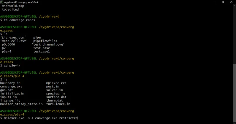
The simulation, after copying the required executables and the license file in the case setup folder, is ran with 4 processor parallely.

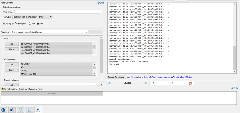
After postconverting the output files in the Converge's built in post processor, as per recognizable format, the contours for velocity and pressure variation are plotted in Converge Line plot tool and ParaView.

Contours:

For grid dx = dy = dz = 0.0006

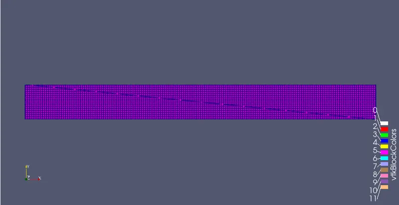
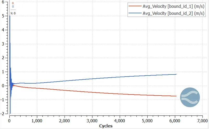
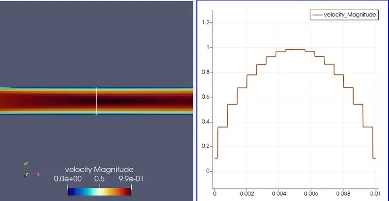
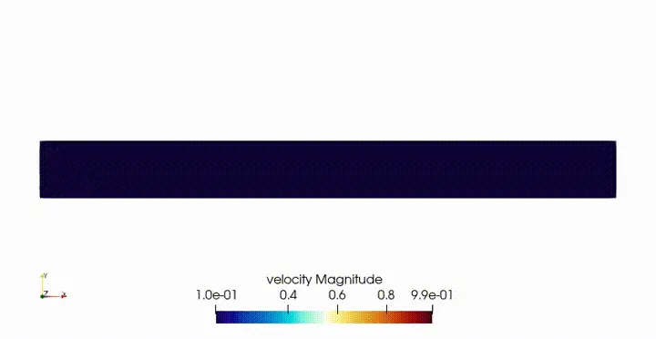
Velocity variation at inlet and outlet

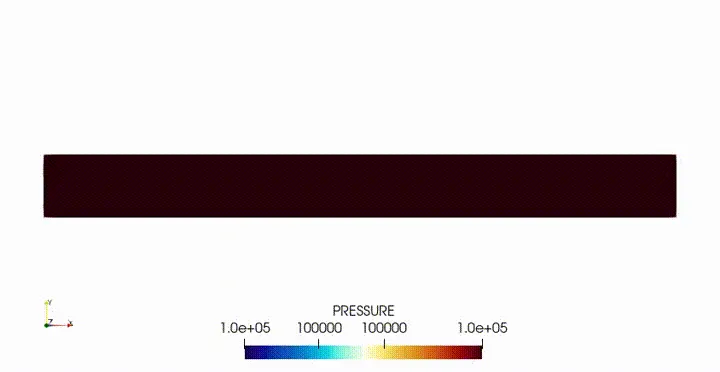
Total pressure variation at inlet and outlet

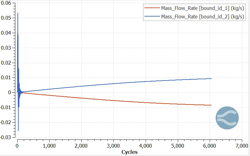
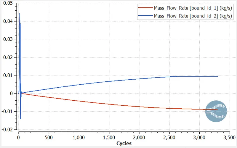
Massflow rate variation at inlet and outlet

For grid dx = dy = dz = 0.00045

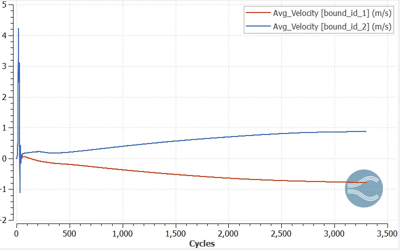
Velocity variation at inlet and outlet

Total pressure variation at inlet and outlet

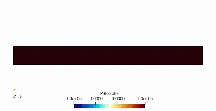
Massflow rate variation at inlet and outlet

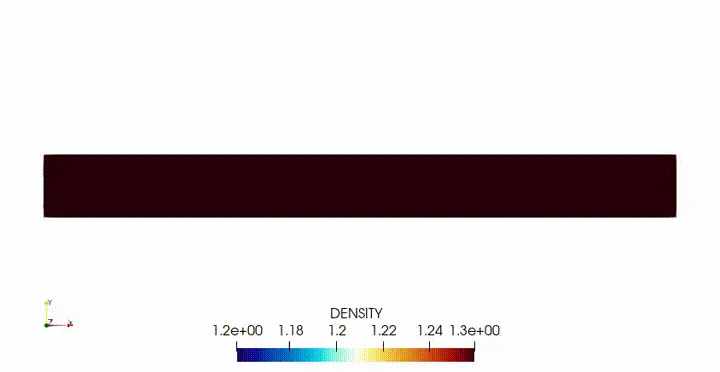
For grid dx = dy = dz = 0.0003

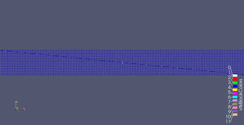
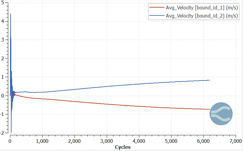
Velocity variation at inlet and outlet

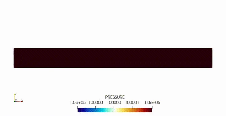
Total pressure variation at inlet and outlet

Massflow rate variation at inlet and outlet

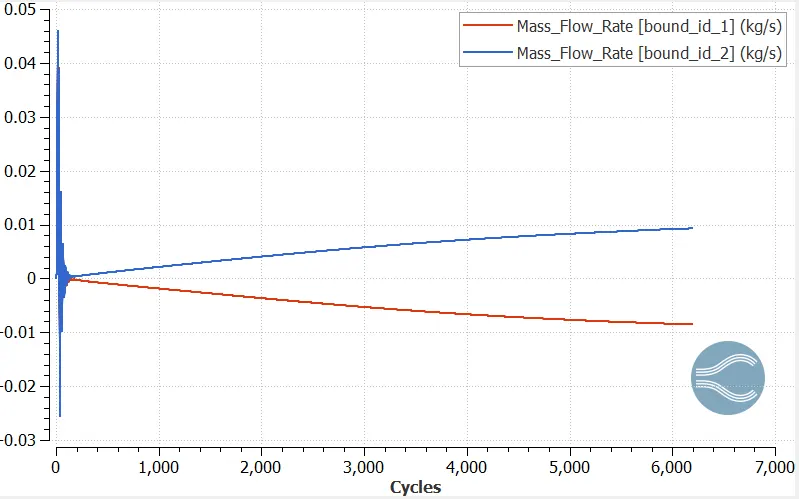
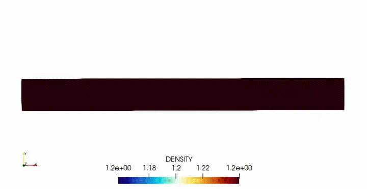
From the above plots, following is noted;

Case	Inlet velocity(m/s)	Outlet velocity(m/s)	Inlet Mass flow rate (kg/s)	Outlet Mass flow rate (kg/s)
1.	0.73	0.81	0.008	0.009
2.	0.78	0.87	0.008	0.009
3.	0.73	0.82	0.008	0.009

Conclusion:

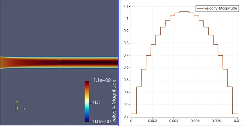
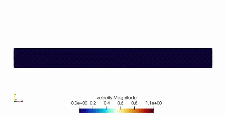
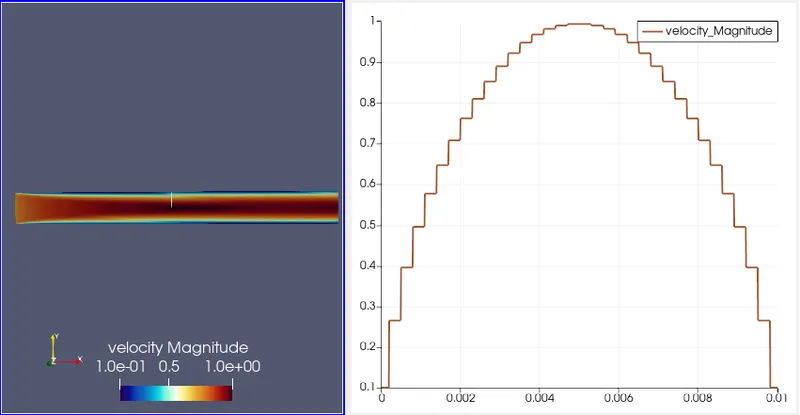
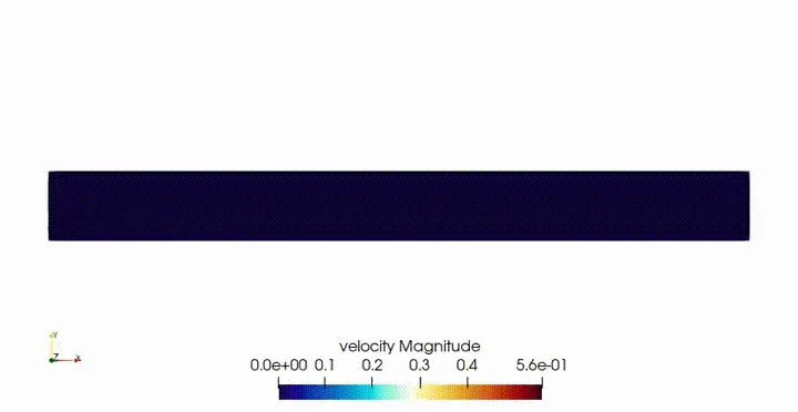
As seen from the velocity animations, the flow at the surface edges has zero velocity as of no slip condition, and as the fluid continues to propogate, its velocity is increased, forming a parabolic velocity profile, which indicates that the maximum velocity is at the centre as the streamlines there are least impacted by the wall friction.

Coming to the parabolic velocity plot, the profile is captured better when the grid size is small, and a good quality of mesh is reliable to appropriate results.

The graphical values of the velocity variation and the mass flow rate indicates that the "Continuity Equation" is conserved locally. amount of