Week 5.1 - Mid term project - Solving the steady and unsteady 2D heat conduction problem
Week 5.1 - Mid term project - Solving the steady and unsteady 2D heat conduction problem
Aim : To visualize the 2D Steady state and Unsteady state (with different techniques) diffusion problem in a domain.
1. Condisering the steady state problem:-
The two dimensional steady state equation is given as,
`(del^2T)/ (delx^2) + (del^2T)/ (dely^2) = 0`
The same equation in the point(iterative)form can be written as,
`Ti,j = 1/k(((Ti-1,j) + (Ti+1,j))/ (Δx^2)) + 1/k(((Ti,j-1) + (Ti,j+1))/ (Δy^2) )`
For the steady state, the program starts by defining number of nodes in x and y directions, as the preassumed domain is a flat plate of 1 meter, and then is discretized. Secondly, the domain's boundary conditions are given as four temperature values, in K, in four sides respectively. Thereafter along with adding the error and the tolerance values, these four sides are assigned as first and last coloumns and top and bottom rows as a bounded square and a 2D array is created.
Now, inside two four loops for x and y, the formula given from 2 to nx-1, as the value of 1st row is known and the process will be upto 24th node (i.e. 25-1 = 24) as the value of last node(25th), is also known. This process will keep on repeateting till the error term drops below the tolerance. Here the old value of temperature needs to be updated else the while loop will not stop, and hence when the error and tolerance criteria is met, the loop will stop meaning that the solution has reached the steady state.
If the Jacobi method is used then the old values of temperature has to be added for '`Ti-1,j`' terms, while if the Gauss-Siedal method is used then intead of old, new values of temperature are to be added. For Successive Over Relaxation method, a relaxation factor (w) is introduced; with under or over-relaxation.
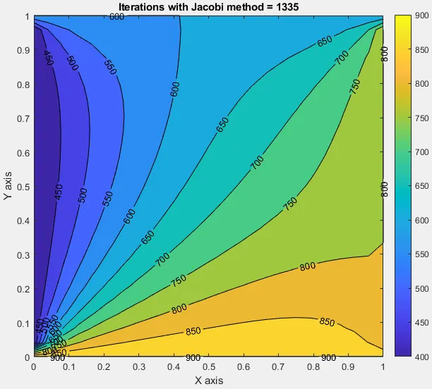
A 2D contour plot, with a coloured specturm is created with sprintf command that shows the number of iterations with each method.
1.1. Program for steady state with Jacobi Method.
clear all
clc
% Let the domain be a 1x1 square metres

%Number of nodes in x and y dir. be 25
nx=25;
ny=nx;
x=linspace(0,1,nx);
y=linspace(0,1,ny);
dx=x(2)-x(1);
dy=y(2)-y(1);
error=9e9;

%Tolerance
tol=1e-4;

%Domain's B.C.'s, temperatues in K
T_L=400;
T_R=800;
T_T=600;
T_B=900;
T=ones(nx,ny);

% Temperature at B.C.'s in K
T(:,1)=T_L;
T(:,end)=T_R;
T(end,:)=T_T;
T(1,:)=T_B;

%Copy of T
[X Y]=meshgrid(x,y);
Told=T;

 % For Jacobi method
 for iterative_solver=1;

    if iterative_solver==1;

        jacobi_iterations=1;
         while (error>tol)
             for i=2:nx-1
                 for j=2:ny-1
                     T(i,j)=0.25*(Told(i-1,j)+Told(i+1,j)+Told(i,j-1)+Told(i,j+1));
                 end
             end
             error=max(max(abs(Told-T)));
             Told=T;
             jacobi_iterations = jacobi_iterations+1;
         end
    end

    figure(1);
    [P,Q]=contourf(X,Y,T);
    clabel(P,Q);
    colorbar;
    title_text=sprintf('Iterations with Jacobi method = %d',jacobi_iterations);
    title(title_text);
    xlabel('X axis');
    ylabel('Y axis');
    fprintf('jacobi=%d/n',jacobi_iterations);
    pause(0.03);

 end
1.2. Program for steady state with Gauss-Siedal Method
clear all
clc
% Let the domain be a 1x1 square metres

%Number of nodes in x and y dir. be 25
nx=25;
ny=nx;
x=linspace(0,1,nx);
y=linspace(0,1,ny);
dx=x(2)-x(1);
dy=y(2)-y(1);
error=9e9;

%Tolerance
tol=1e-4;

%Domain's B.C.'s, temperatues in K
T_L=400;
T_R=800;
T_T=600;
T_B=900;
T=ones(nx,ny);

% Temperature at B.C.'s in K
T(:,1)=T_L;
T(:,end)=T_R;
T(end,:)=T_T;
T(1,:)=T_B;

%Copy of T
[X Y]=meshgrid(x,y);
Told=T;

 % For Gauss-Siedal method
 for iterative_solver=2;

     if iterative_solver==2;

        gs_iterations=1;
         while (error>tol)
             for i=2:nx-1
                 for j=2:ny-1
                     T(i,j)=0.25*(T(i-1,j)+Told(i+1,j)+T(i,j-1)+Told(i,j+1));
                 end
             end
             error=max(max(abs(Told-T)));
             Told=T;
             gs_iterations = gs_iterations+1;
         end
    end

    figure(1);
    [P,Q]=contourf(X,Y,T);
    clabel(P,Q);
    colorbar;
    title_text=sprintf('Iterations with Gauss-Siedal method = %d',gs_iterations);
    title(title_text);
    xlabel('X axis');
    ylabel('Y axis');
    fprintf('gs=%d/n',gs_iterations);
    pause(0.03);

 end
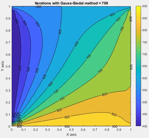
1.3. Program for steady state with S.O.R. Method
clear all
clc
% Let the domain be a 1x1 square metres

%Number of nodes in x and y dir. be 25
nx=25;
ny=nx;
x=linspace(0,1,nx);
y=linspace(0,1,ny);
dx=x(2)-x(1);
dy=y(2)-y(1);
error=9e9;

%Tolerance
tol=1e-4;

%Domain's B.C.'s, temperatues in K
T_L=400;
T_R=800;
T_T=600;
T_B=900;
T=ones(nx,ny);

%Calculating relaxation factor
omega=2/(1+sin(pi*dx));

% Temperature at B.C.'s in K
T(:,1)=T_L;
T(:,end)=T_R;
T(end,:)=T_T;
T(1,:)=T_B;

%Copy of T
[X Y]=meshgrid(x,y);
Told=T;

 % For SOR method
 for iterative_solver=3;
     if iterative_solver==3;
        SOR_iterations=1;
         while (error>tol)
             for i=2:nx-1
                 for j=2:ny-1
                     T(i,j)=((1-omega)*Told(i,j)+(omega*0.25*(T(i-1,j)+Told(i+1,j)+T(i,j-1)+Told(i,j+1))));
                 end
             end
             error=max(max(abs(Told-T)));
             Told=T;
             SOR_iterations = SOR_iterations+1;
         end
    end

    figure(1);
    [P,Q]=contourf(X,Y,T);
    clabel(P,Q);
    colorbar;
    title_text=sprintf('Iterations with SOR method = %d',SOR_iterations);
    title(title_text);
    xlabel('X axis');
    ylabel('Y axis');
    fprintf('SOR=%d/n',SOR_iterations);
    pause(0.03);

 end
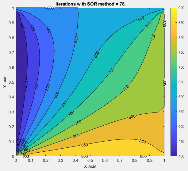
From the above three 2D plots, it is clear that the number of iterations reaching the steady state were highest for Jacobi Method, they were less for Gauss-Siedal Method, while SOR Method had least iterative steps, giving out that SOR faster method than the other two.
2. Condisering the unsteady state problem:-
The two dimensional steady state equation, having a time derivative term is given as,
`(delT)/(delt) = alpha((del^2T)/ (delx^2) + (del^2T)/ (dely^2))`
In the point iterative form the expression is as,
`(Tp^(n+1) - Tp)/(Δt) = alpha((Tl - 2Tp+Tr)/(Δx^2) + (Tt - 2Tp+Tb)/(Δy^2))`
where, Tp = temperature at current point, K
Tl and Tr = temperature at left and right nodes respectively, K
Tt and Tb = temperature at top and bottom nodes respectively, K
From the above iterative equation, the R.H.S. of the term excluding α, can be computed at either 'nth(or with Explicit scheme)' or '(n+1)th (or Implicit scheme)' timestep.
2.1 Solving with 'nth' or Explicit scheme with no iterative solvers
In this case, the final point iterative expression is given as;
`Tp^(n+1) = Tp^n + k1(Tl - 2Tp+Tr)^n + k2(Tt - 2Tp+Tb)^n`
where k1 = `alpha ((Δt)/(Δx^2))`= CFL number in x direction`
k2 = `alpha ((Δt)/(Δy^2))`= CFL number in y direction`
In unsteady state program starts by defining number of nodes in x and y directions, as the preassumed domain is a flat plate of 1 meter, and then is discretized. Secondly, the domain's boundary conditions are given as four temperature values, in K, in four sides respectively. Thereafter along with adding the error, tolerance value, CFL number and time step size, these four sides are assigned as first and last coloumns and top and bottom rows as a bounded square and a 2D array is created. In the next step the ki and k2 as two CFL numbers in x and y directions are introduced.
Inside the for loops the iterative equation is splitted in three terms and is added, with an updation of old value of temperature. For the diffusion problem to solve by the explicit method, the total CFL number should be less than or equal to 0.5, if it is more than 0.5 solution will be unstable.
2.1 Program for unsteady state by explicit method
% 2D Unsteady Conduction equation by Explicit Method
% Let the domain be a 1x1 square metres

%Number of nodes in x and y dir. be 25
nx=25;
ny=nx;
x=linspace(0,1,nx);
y=linspace(0,1,ny);
dx=x(2)-x(1);
dy=y(2)-y(1);
error=9e9;

%Tolerance
tol=1e-4;
dt=0.1;

%Convective coefficient
alpha = 1e-3;
t=200;

%CFL number
CFL = alpha*dt/(dx^2);

%Domain's B.C.'s, temperatues in K
T_L=400;
T_R=800;
T_T=600;
T_B=900;

% Temperature at B.C.'s in K
T(:,1)=T_L;
T(:,end)=T_R;
T(end,:)=T_T;
T(1,:)=T_B;

% CFL numbers in X and Y dir.
k1=(alpha*dt)/(dx^2);
k2=(alpha*dt)/(dy^2);

% Copy of T
[X Y]=meshgrid(x,y);
Told=T;
nt=t/dt;

%2D Unsteady state heat conduction equation in explicit method
for v=1:nt
       for i=2:nx-1
               for j=2:ny-1
                   term1=Told(i,j);
                   term2=k1*(Told(i+1,j)-2*Told(i,j)+Told(i-1,j));
                    term3=k2*(Told(i,j+1)-2*Told(i,j)+Told(i,j-1));
                    T(i,j)=term1+term2+term3;
               end
       end
   %Updating old temerature
          Told=T;
   end

    figure(1);
    [P,Q] = contourf(X,Y,T);
    clabel(P,Q);
    colorbar;
    title_text=sprintf('Explicit method');
    title(title_text);
    xlabel('X axis');
    ylabel('Y axis');
pause(0.03); 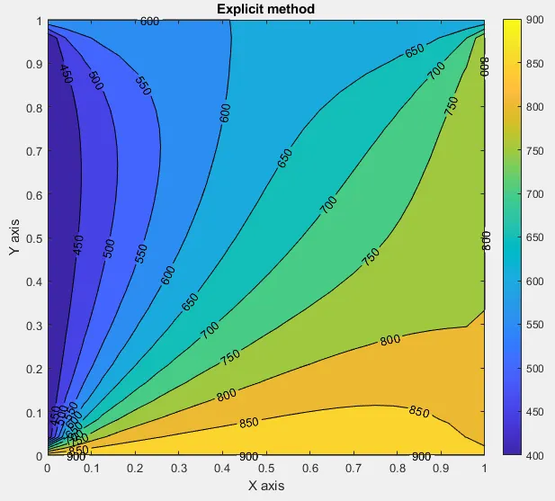
2.2 Solving with '(n+1)th' or Implicit scheme with iterative solvers
In this case, the final point iterative expression is given as;
`Tp^(n+1) = (1/(1+2k1+2k2))(Tp^n + k1(Tl+Tr)^(n+1) + k2(Tt +Tb)^(n+1))`
where k1 = `alpha ((Δt)/(Δx^2))`= CFL number in x direction`
k2 = `alpha ((Δt)/(Δy^2))`= CFL number in y direction
Solving for this equation with implicit method, iterative methods are required. Here in iterative methods, in the loops the 'T_prev' value is for previous timesteps and the updating 'T_old' value is for previous iterations, for solving (n+1)th temperature values. After the error term finds the difference between the old and present temperature values, till the error drops below tolerance. As when the solution gets converged, the 'T_prev' value is upgraded to the initial one for the next time step.
2.2.a Program for 2D unsteady equation with Jacobi Method
%2D Unsteady state equation by Implicit Method

%Number of nodes in x and y dir. be 25
nx=25;
ny=nx;
x=linspace(0,1,nx);
y=linspace(0,1,ny);
dx=x(2)-x(1);
dy=y(2)-y(1);
error=9e9;

%Tolerance
tol=1e-4;
dt=0.1;

%Convective coefficient
alpha = 1;
t=200;

%CFL number
CFL = alpha*dt/(dx^2);

%Domain's B.C.'s, temperatues in K
T_L=400;
T_R=800;
T_T=600;
T_B=900;
T=298*ones(nx,ny);

% Temperature at B.C.'s in K
T(:,1)=T_L;
T(:,end)=T_R;
T(end,:)=T_T;
T(1,:)=T_B;

% CFL numbers in X and Y dir.
k1=(alpha*dt)/(dx^2);
k2=(alpha*dt)/(dy^2);
nt=t/dt;

% Copy of T
[X Y]=meshgrid(x,y);
Told=T;
T_prev_dt=Told;

   %2D unsteady heat conduction equation by Jacobi Method
   nt=t/dt;
   iterative_solver=1;
   jacobi_iterations=1;
   for v=1:nt
       if iterative_solver==1
           term1=(1+2*k1+2*k2)^(-1);
           term2=k1*term1;
           term3=k2*term1;

           error=100;
           while(error>tol)
               for i=2:nx-1
                   for j=2:ny-1
                       H=(Told(i-1,j)+Told(i+1,j));
                       V=(Told(i,j-1)+Told(i,j+1));
                        T(i,j)=(T_prev_dt(i,j)*term1)+(H*term2)+(V*term3);
                   end
               end
               error=max(max(abs(Told-T)));
               Told=T;
               jacobi_iterations=jacobi_iterations+1;
           end
           T_prev_dt=T;
       end

    figure(1);
    [P,Q] = contourf(X,Y,T);
    clabel(P,Q);
    colorbar;
    title_text=sprintf('Iterations by Jacobi Method = %df',jacobi_iterations+1,CFL');
    title(title_text);
    xlabel('X axis');
    ylabel('Y axis');
    pause(0.03);
   end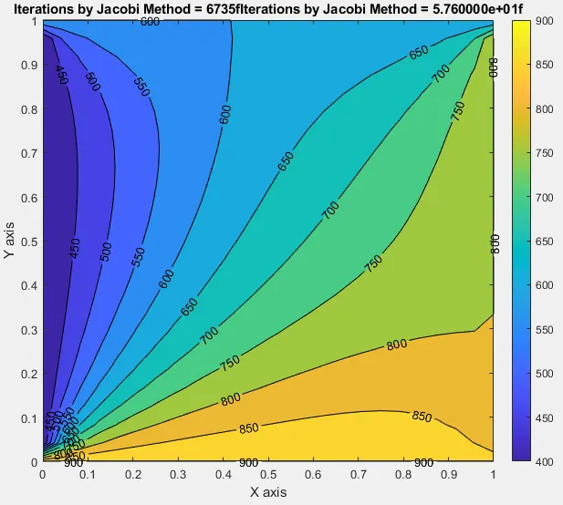
2.2.b Program for 2D unsteady equation with Gauss-Siedal Method
%2D Unsteady state equation by Implicit Method

%Number of nodes in x and y dir. be 25
nx=25;
ny=nx;
x=linspace(0,1,nx);
y=linspace(0,1,ny);
dx=x(2)-x(1);
dy=y(2)-y(1);
error=9e9;

%Tolerance
tol=1e-4;
dt=0.1;

%Convective coefficient
alpha = 1;
t=200;

%CFL number
CFL = alpha*dt/(dx^2);

%Domain's B.C.'s, temperatues in K
T_L=400;
T_R=800;
T_T=600;
T_B=900;
T=298*ones(nx,ny);

% Temperature at B.C.'s in K
T(:,1)=T_L;
T(:,end)=T_R;
T(end,:)=T_T;
T(1,:)=T_B;

% CFL numbers in X and Y dir.
k1=(alpha*dt)/(dx^2);
k2=(alpha*dt)/(dy^2);
nt=t/dt;

% Copy of T
[X Y]=meshgrid(x,y);
Told=T;
T_prev_dt=Told;

%2D unsteady heat conduction equation by Gauss-Siedal Method
   iterative_solver=2;
    gs_iterations=1;
    for w=1:nt
       if iterative_solver==2
            term1=(1+2*k1+2*k2)^(-1);
            term2=k1*term1;
            term3=k2*term1;

           error=100;
            while(error>tol)
                for i=2:nx-1
                    for j=2:ny-1
                        H=(T(i-1,j)+Told(i+1,j));
                        V=(T(i,j-1)+Told(i,j+1));
                         T(i,j)=(T_prev_dt(i,j)*term1)+(H*term2)+(V*term3);
                   end
               end
                error=max(max(abs(Told-T)));
                Told=T;
                gs_iterations=gs_iterations+1;
            end
        T_prev_dt=T;
        end

     [P,Q] = contourf(X,Y,T);
     clabel(P,Q);
     colorbar;
     title_text=sprintf('Iterations by Gauss-Siedal Method = %d',gs_iterations,CFL');
     title(title_text);
     xlabel('X axis');
     ylabel('Y axis');
     pause(0.03);
    end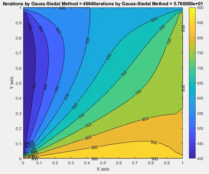
2.2.c Program for 2D unsteady equation with S.O.R. Method
%2D Unsteady state equation by Implicit Method

%Number of nodes in x and y dir. be 25
nx=25;
ny=nx;
x=linspace(0,1,nx);
y=linspace(0,1,ny);
dx=x(2)-x(1);
dy=y(2)-y(1);
error=9e9;

%Tolerance
tol=1e-4;
dt=0.1;

%Convective coefficient
alpha = 1;
t=200;

%CFL number
CFL = alpha*dt/(dx^2);

%Calculating relaxation factor
omega=2/(1+sin(pi*dx));

%Domain's B.C.'s, temperatues in K
T_L=400;
T_R=800;
T_T=600;
T_B=900;
T=298*ones(nx,ny);

% Temperature at B.C.'s in K
T(:,1)=T_L;
T(:,end)=T_R;
T(end,:)=T_T;
T(1,:)=T_B;

% CFL numbers in X and Y dir.
k1=(alpha*dt)/(dx^2);
k2=(alpha*dt)/(dy^2);
nt=t/dt;

% Copy of T
[X Y]=meshgrid(x,y);
Told=T;
T_prev_dt=Told;

%2D unsteady heat conduction equation by SOR Method
iterative_solver=3;
SOR_iterations=1;
    for Z=1:nt
        if iterative_solver==3
            term1=(1+2*k1+2*k2)^(-1);
            term2=k1*term1;
            term3=k2*term1;

            error=100;
            while(error >tol)
                for i=2:nx-1
                    for j=2:ny-1
                        H=(omega*T(i-1,j)+(1-omega)*Told(i-1,j)+Told(i+1,j));
                        V=(omega*T(i,j-1)+(1-omega)*Told(i,j-1)+Told(i,j+1));
                        T(i,j)=(T_prev_dt(i,j)*term1)+(H*term2)+(V*term3);
                    end
                end
               error=max(max(abs(Told-T)));
                Told=T;
                SOR_iterations=SOR_iterations+1;
            end
        T_prev_dt=T;
        end

    [P,Q] = contourf(X,Y,T);
    clabel(P,Q);
    colorbar;
     title_text=sprintf('Iterations by SOR Method = %d',SOR_iterations,CFL');
     title(title_text);
     xlabel('X axis');
     ylabel('Y axis');
     pause(0.03);
end 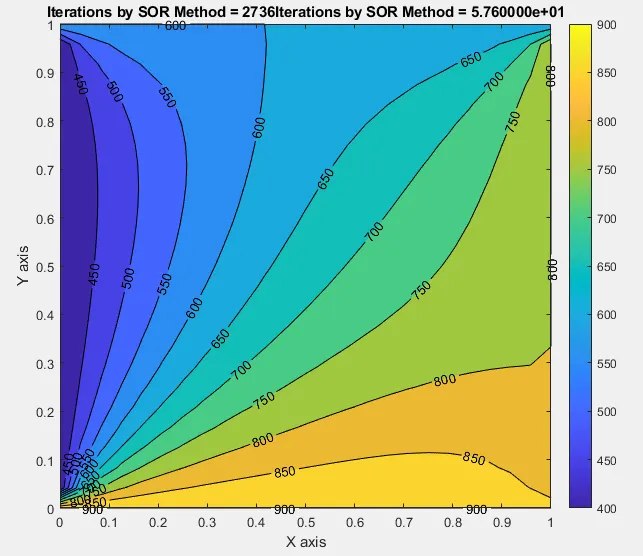
From the above 2D plots, it is clear that explicit method is way mor faster in processing as compared to the three implicit iterative methods. In case of the implicit methods, still with the iterations, the S.O.R. method is more accurate than the other two methods for solving an unsteady 2D heat conduction problem.