MATLAB-Final Independent Project
PROJECT TITLE : Calculation of the steady flight parameters and performance prediction of an UCAV
AIM : To determine the change in variables during an un-accelerated flight.
OBJECTIVE : The primary emphasis lies on calculation of various data and making assumptions of a few.
METHODOLOGY : For the present work, in order to plot the variations, the data required for the procurement is retrieved from online resources, thereafter, it is included for continuing the further work.
- Introduction:
The magnitude of the significance, however depends on required analysis and accuracy, presently it is a rough prediction of the performance data of an UCAV, with more focus on the theoretical basis.
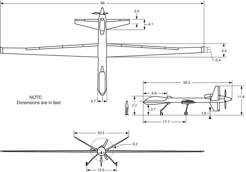
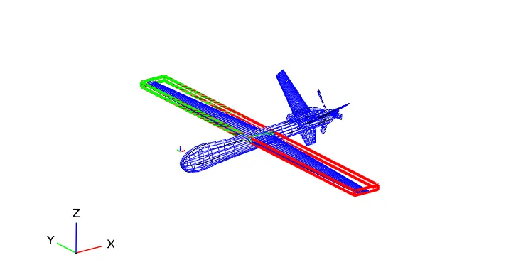
To begin with, for purpose, the General Atomics MQ-9A UCAV drone, has been chosen having the following configuration[1],
| Variables | Symbol | Unit |
| Net takeoff weight | `W` | 4760 `kg` |
|
Wingspan
|
`b` | 20 `m` |
|
Root chord
|
`cr` | 1.6459 `m` |
|
Tip chord
|
`ct` | 0.7315 `m` |
|
Mean wing chord
|
`MAC` | 1.247 `m` |
|
Wing reference area
|
`Sref` | 22.48 `m^2` |
| Aspect ratio | `AR` | 17.80 |
- Steady flight analysis
- For any flight vehicle, the main source of lift generation is the wing, though horizontal stablizers are for llft corrections. The root and tip sections of the MQ-9A Reaper, is implemented with MH114 airfoil[2],
- Program:
% Specifications of MQ-9A UCAV

Wnet = 4760;
MAC = 1.2470;
Sref = 22.48;
AR = 17.80;
wl = linspace(10,1,100);

% Velocity range in m/s
v = [31:130];            % Max. limit is upto 133 m/s

% Atmospheric variables at 2000 m under I.S.A.
rho = 0.8217;         % Density in kg/m^3
p = 0.7950            % Pressure in kPa
vu = 1.715e-5;        % Kinematic viscosity in m^2/s
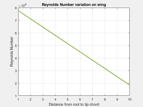
Re = (rho*v*MAC)/vu;  % Reynold's number as per velocity range
A = 332.5;            % Sound speed in m/s
M = v/A;              % Mach number variation


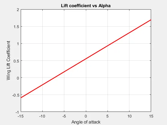
% The 3D Lift curve slope, or wing's is
e = 0.8;                          % efficiency same for airfoil and wing
a0 = 0.0844;                      % lcs of MH114
a = a0/(1 + (57.3*a0/(pi*e*AR))); % lcs of MH114 wing
alpha0= -7.25;                    % angle @Cl_MH114 = 0

% To find Cl(WING) vs Alpha
alpha = linspace(-15,15,100);
CL=a*(alpha-alpha0);

% PLot of CL(wing) vs Alpha
figure(1);
plot(alpha ,CL ,'linewidth',2, 'color','r');
xlabel('Angle of attack')
ylabel('Wing Lift Coefficient')
title('Lift coefficient vs Alpha')
grid on

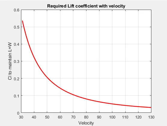
% Required Lift coefficient with angle
figure(2);
C_L = 2*Wnet./(rho*Sref*v.^2);
plot(v ,C_L ,'linewidth',2, 'color','r');
xlabel('Velocity');
ylabel('Cl to maintain L=W');
title('Required Lift coefficient with velocity')
grid on

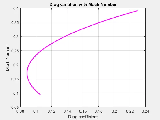
figure(3)
plot(CD, M ,'linewidth',2,'color', 'm')
xlabel('Drag coefficient');
ylabel('Mach Number');
title('Drag variation with Mach Number')
grid on

figure(4)
plot(wl, Re ,'linewidth',2,'color', '[0.4660 0.6740 0.1880]')
xlabel('Distance from root to tip chord');
ylabel('Reynolds Number');
title('Reynolds Number variation on wing')
grid on

% Drag calculation and plotting
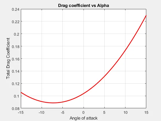
CD0 = 0.08866;              % Parasite drag coefficient overall
CDi = CL.^2/(pi*AR*e);      % Induced drag coefficient
CDf = 1.2*CDi               % Fuselage drag estimation
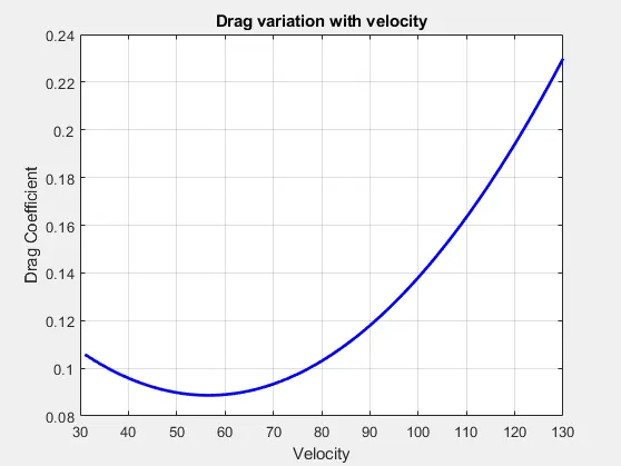
CD = CD0 + CDi + CDf;       % Total drag coefficient

figure(5)
plot(alpha ,CD ,'linewidth',2, 'color','r')
xlabel('Angle of attack');
ylabel('Total Drag Coefficient');
title('Drag coefficient vs Alpha')
grid on

figure(6)
plot(v, CD, 'linewidth', 2,'color','b')
xlabel('Velocity')
ylabel('Drag Coefficient')
title('Drag variation with velocity')

grid on

% To ovrecome Drag force,
D = 0.5*rho*v.^2*Sref.*CD;
T =D;

figure(7)
plot(v, T,'linewidth',2,'color', 'y')
xlabel('Velocity');
ylabel('Thrust required(Newtons)');
title('Thrust vs velocity')
grid on

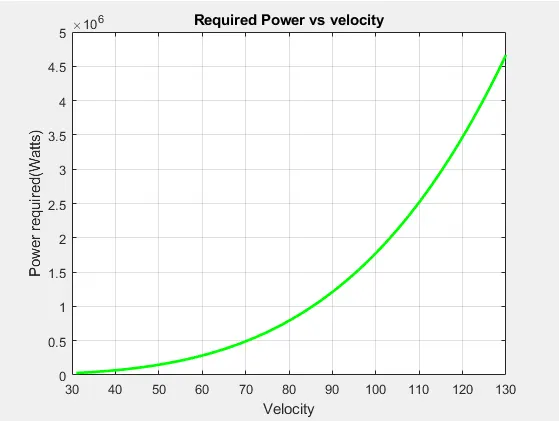
% Net Power Required, for given configuration
PREQ = power_req(4760 ,0.8217, 22.48)

figure(8)
plot(v, PREQ,'linewidth',2,'color', 'g')
xlabel('Velocity');
ylabel('Power required(Watts)');
title('Required Power vs velocity')
grid on
- Function:
function [Power] = power_req(Wnet,rho, Sref)

CD = linspace(0.105795270359314,0.229896708133328, 100);
v = [31:130]
Power = 0.5*rho*v.^2*Sref.*CD.*v;

end