Week 4 - CHT Analysis on Exhaust port
Introduction to GUI based CFD using Ansys Fluent
Week - 4 : CHT Analysis on Exhaust port
CHT Analysis:
Conjugate Heat Transfer involves exchange of thermal energy between fluid and solid interface. Such analysis is carried out for heat exchangers, cooling of electronic equipments, cooling and heating systems, exhaust manifolds and components where convective phenomena is of significance.
In any fluid solid interaction, whenever there is flow of fluid at surface, there is formation of thermal boundary layer inculcating the energy exchange between surface and fluid, CHT is taken into picture to determine and analyse the Heat transfer occuring. The current project is about CHT analysis of an exhaust manifold of an engine, thereby to determine the convective heat transfer coefficient.
Analysis setup:
The CAD model of an exhaust manifold is loaded in Ansys Spaceclaim, and the faces and other geometry is categorized in various named selections. There are total four inlets, indicated with blue arrows and one outlet by red arrow, following the mass conservation equation.
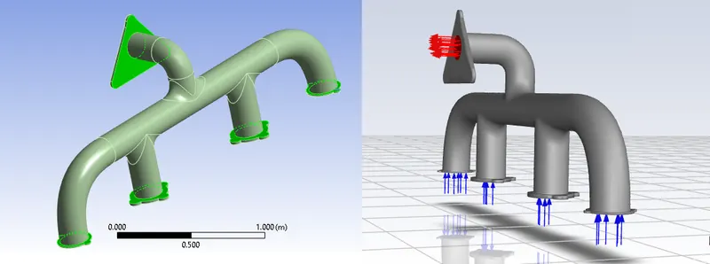
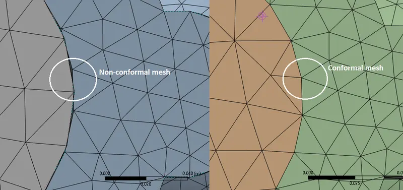
The green parts showed for the geometry is given the adiabetic condition meaning that there is no heat transfer involver at those regions. Following up with the next stage, the model is loaded in Mesh module where entire geometry is discretized by sharing topology as to pass on the information from adjacent boundary to cells.
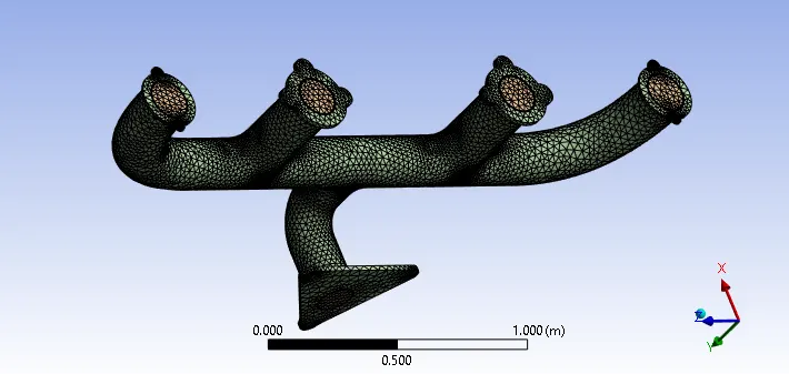
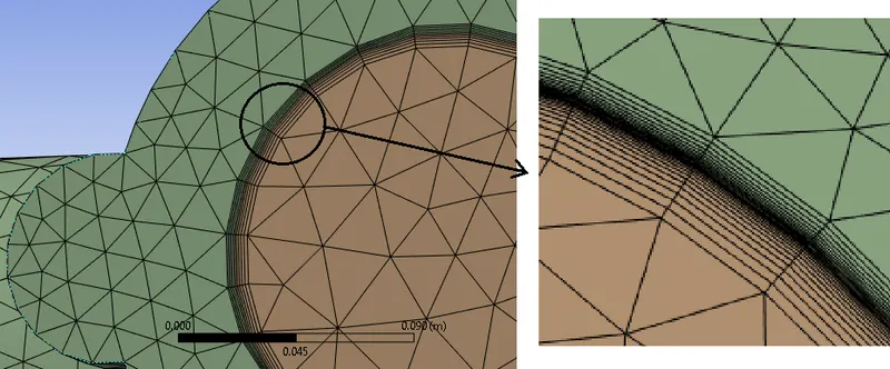
With this, the inflation layers are created at the walls to capture the viscous interaction of fluid flow.
Secondly in the Ansys Fluent module, the Pressure based solver is used as the flow has very less velocity and the density does not vary significantly. The solver solves the corrected values of pressure and velocity for convergence, Continuity equation, x-momentum, y-momentum and z-momentum equation. Since the flow of air takes place at 700 Kelvin, the Energy Equation is accounted as well. The boundary conditions, fluid and properties of the solid are as follows;
| Solid | Aluminium |
| Density (`rho`) | 2719 `(kg)/m^3` |
| Specific heat (Cp) | 871 `(J)/(kg K)` |
| Conductivity | 202.4 `(W)/(m K)` |
| Fluid | Air |
| Density (`rho`) | 1.225 `(kg)/m^3` |
| Specific heat (Cp) | 1006.43`(J)/(kg K)` |
| Conductivity (k) | 0.0242 `(W)/(m K)` |
| Dynamic viscosity `(mu)` | 0.0000146 `(m^2)/s` |
| Kinematic viscosity (v) | 1.7894 `(kg m)/s` |
| Characteristic length (inlet diameter) 'd' | 0.166 m |
| Reynolds Number (Re) | 69640 |
Boundary Condition
| Inlet | Velocity = 5m/s, Temperature = 700 K |
| Outlet | Atmospheric pressure, 1 atm |
| Wall (outer) | Convection |
| Other walls | No-Slip |
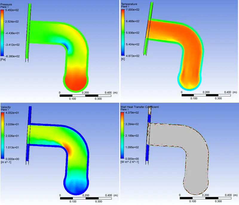
By usind Hybrid initialization, the initial temperature values are printed out, and the surface heat transfer coefficient at inner wall is illustrated by creating a section plane normal to Z axis.
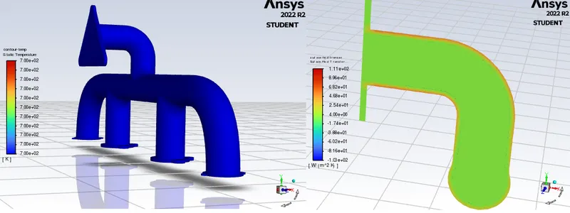
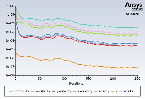
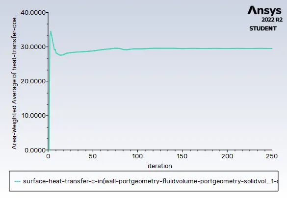
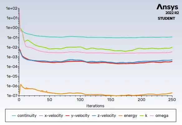
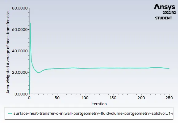
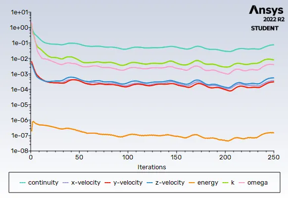
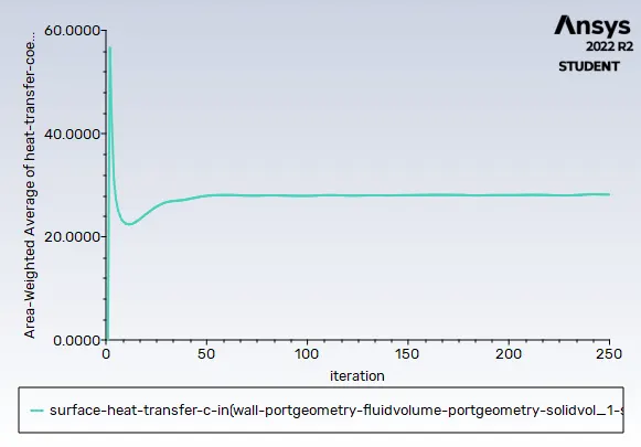
The plots for residuals and inner wall's heat transfer coefficient are created and since the flow is viscous at wall, different turbulence models are selected for the simulation purpose.
In order to capture the flow parameters at the boundary, it is important to set up the mesh such that it gives the appropriate predictions.
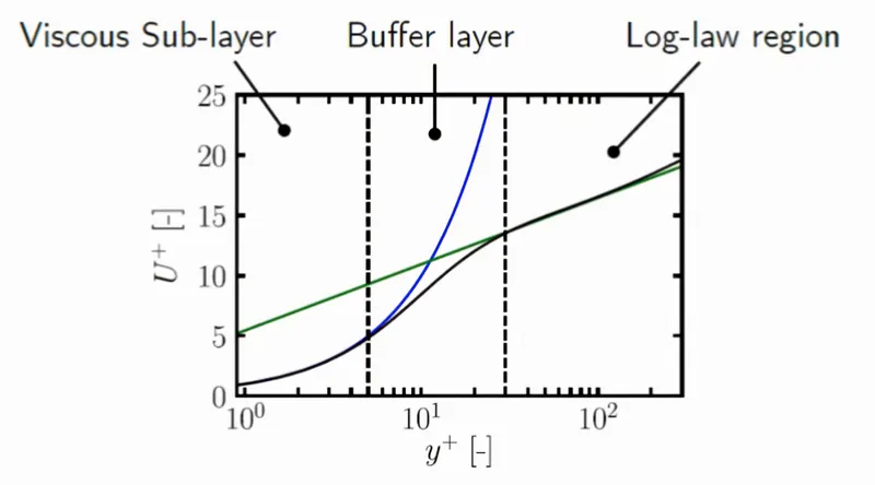
U+ is the ratio of mean component of velocity and friction velocity whereas the y+ is the non-dimentional distance from the wall. The y+ values in the buffer region are not suitable for input for calculating the nearest distance of cell from the wall. The reason for the same is the velocity profile (curve) being not well defined, does not give suitable results as within this specific region the law is not followed for either of viscous region or of outer region.
For modelling the mesh near the wall, the wall functions incorporated defines the first cell height off the wall instead of creating a gradually dense mesh.
With the desired y+ values, the wall spacing or the distance of first cell from the wall can be calculated using follwing relation:
`y+ = (rho*v**yp)/(mu)`
where `v** = sqrt(tau/rho)`, `tau = 0.5*rho*Cf*v^2`
For internal flows, `Cf = 0.079⋅Re^(−0.2)`
Here `yp` = distance of first cell from wall
`tau`= shear stress (`N/(m^2)`)
`Cf`= Skin-friction coefficient
The simulation is run for k-omega model having suitability of y+ from 1 to 5 and for k-epsilon model with `30< y+<300`.
Plots:
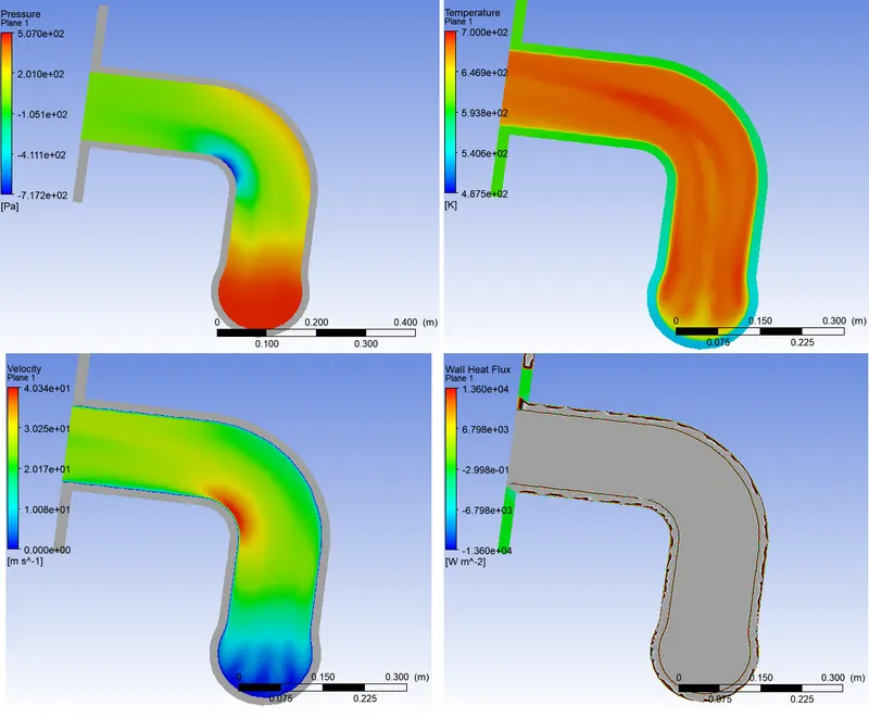
With k-epsilon model, having y+ = 70
With k-omega model, having y+ = 1
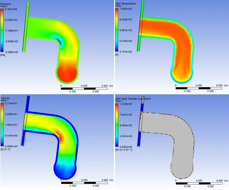
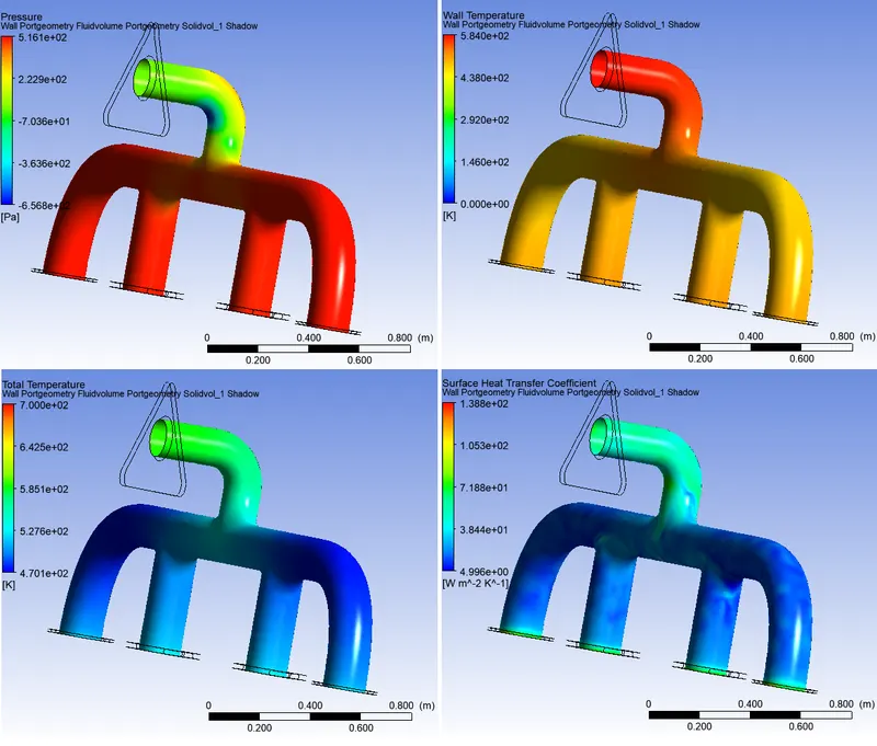
With k-omega model, having y+ = 3
Performing above calculations, following is noted;
| y+ | Model |
Inflation layers |
Cells | yp |
Heat transfer coefficient |
| 1 | k-omega SST | 9 | 333810 | 5.573e-5 | 24.24 |
| 3 | k-omega SST | 9 | 326556 | 1.671e-4 | 28.02 |
| 5 | k-omega Std. | 9 | 320795 | 2.786e-4 | 29.31 |
| 1 | k-omega Std. | 12 | 403406 | t = 0.0059 m | 28.91 |
| 30 | k-epsilon | 12 | 392225 | 1.671e-3 | 28.76 |
| 70 | k-epsilon | 9 | 255086 | 3.901e-3 | 29.37 |
Conclusion:
Being defined the values of y+ from both the models, the value of Convective heat tranfer coefficient for k-omega model fluctuates aruund 28, whilst, for k-epsilon model is near to 28.5 `W/(m^2K)`
The accuracy of the prediction depends on the number of inflation layers created above the wall, number of cells (for better approximations), viscous model with appropriate wall treatment, quality of mesh as with high value of y+, the distance from the wall of yp increases, this sometimes make certain cells skewed.
Another reason for the variation of heat transfer co-efficent's values is the total number of cells, this affects the solution time as it is dependent on computation power.
References: