Week 5 - Turbulence modelling challenge

Week 5 - Turbulence Modelling challenge

Attaining the Critical Reynolds Number in a flow, the 'Energy Cascading' takes place, where the larger eddies break down to smaller eddies.

* Types of eddies:

• Large eddies

Their size is proportional to ratio of (Characteristic length/ Free stream velocity);

`size prop (L/(U∞))`

They draw the energy from the mean flow.

• Small eddies

Their size is proportional as, `size prop L/(Re^(3/4))`.

Their energy source is the large eddies.

* Scale of eddies:

• Kolmogrov's Length scale

Larger eddies have a relation as seen above but for determining the size of smaller eddies, below relation can be considered;

`eta = (v^3/epsilon)^(1/4)`

Here , `eta =` Kolmogrov Length scale

`v =` Kinematic viscosity (`m^2/s`)

`epsi=` TKE dissipation rate `(U^3/L)`

• Kolmogrov's Time scale

Used to determine the turn over time of a particular eddie.

`tn = (v/epsi)^(1/2)`

Taking the ratio of length scales of Largest and Smallest eddies;

`L/eta = L/(v^3/epsi)^(1/4)`

Now manipulating the above relation and substituting the value of `epsi`, we have;

`L/eta = Re^(3/4)`

1. Direct Numerical Simulation (DNS):

Solves the N-S Equations at a very small scale, and as per the Kolmogrov's length scale for small eddies.

`eta prop 1/(Re)^(3/4)`

So the grid size must be smaller than above relation, which is too small.

In 3D flow, each dimension of the element must be smaller than the length determined from the Kolmogrov's scale, with 3 dimensions, volume will be;

`Volume prop 1/(Re)^(9/4)`, as this is extensively small magnitude.

Consider if the geometry has a volume '`V`', with the volume of the smallest element as '`Δ V`'.

So total elements; `V/(Δ V)`

Then the total number of elements will be proportional to `Re^(9/4)`.

Thus there will be large number of 3D elements, which makes this method next to impossible to be utilized for industrial applications, however for research purpose, it can be run in 2D.

2. Large Eddy Simulation (LES):

As the name itself suggests, this approach is for resolving the large eddies.

Small eddies are usually modelled by Subgrid scale model.

Here, the number of elements is not as large since the Length scale is dependent on Length and Velocity.

LES is applicable for modelling 'Combustion' and 'Acoustic' phenomena.

"With regards to model the turbulence, Reynold's averaging is applied to the N-S Equations in order to obtain the Reynolds stress terms, for modelling."

Certain Viscous models require additional equations to solve the Reynolds stress terms.

RANS based Viscous Models used are:

3. First Order Models:

These models assume an analogy between laminar and turbulent flows. Models use first order PDEs to solve for turbulent viscosity. These models are categorized as;

• Zero Equation Model

As the name implies, there is no PDE in zero equation models that represents the transfer of turbulent stresses and fluxes, and so it fails to capture the transient behaviour of turbulent viscosity.

It solves the turbulent viscosity directly and is based on Prandtl's Mixing length theory. The Mixing Length model assumes the eddy viscosity terms to be dimensionally similar to Kolmogrov's length and velocity scale.

• One Equation Model

One and Two equations model utilizes RANS decomposition, basically separating fluctuating variable into an 'average' and 'fluctuating' quantities, it is also defined as Time averaging.

The One Equation model is also called Spalart-Allmaras model,

Here PDE is used to solve the TKE for obtaining the Turbulent viscosity. TKE is determined using;

`K = 1/2(bar u^2+bar v^2+bar w^2)`

Thereafter the Turbulent viscosity is determined by, `mut = CsqrtK*lm`.

This viscosity is then substituted in RANS.

It is designed specifically for internal and external aerospace applications involving wall-bounded flows on a fine near-wall mesh. Suitable for large meshed geometries and boundary layer flows under pressure gradient, e.g. airfoils, wings, missiles, transonic cases, etc. It is not suitable for flows under strong pressure gradients.

• Two Equation Model

Here the turbulent viscosity is modelled and utilizes two PDEs to solve for,

a) TKE and Turbulent Dissipation rate

b) TKE and Specific Dissipation rate

These models include k-epsilon and k-omega.

1. Standard k-epsilon

k and ε are solved by the basic two-transport-equation model. This is the k–ε model by default. Coefficients are obtained empirically and are only applicable to completely turbulent flows. It accounts for compressibility, buoyancy, and viscous heating.

It is most widely used and wall functions to calculate ε near walls.

It has good convergence and is memory efficient. Suitable for attached turbulent flow, external flows around complex bodies.

It performs poorly for separated flows.

2. RNG k-epsilon

Coefficients and equations are obtained analytically. Modifying the ε equation significantly enhances the model's capacity to represent extremely stressed flows. The prediction of low Reynolds number and whirling flows is aided by additional alternatives.

Solves for some constraints on Reynolds Stresses.

Appropriate for complex shear flows such boundary layer separation, huge separation, vortex shedding behind bluff bodies, stall in wide-angle diffusers, and room ventilation that involve rapid strain, mild swirl, vortices, and locally transitional flows.

3. Realizable k-epsilon

ε is improved, and effect of swirl is introduced. It used empirical relations to find a modified version of Prandtl Number.

It has practically the same advantages and uses as RNG k-epsilon, possibly easier to converge and more precise than RNG k-epsilon.

4. Standard k–ω

k-omega models does not contain terms undefined at the wall, here Wall Functions (discussed afterwards) are not required at the wall.

It shows good behaviour in wall bounded and low Reynolds Number flows. It is suitable to predict the flow transition and can be considered in the case of free shear flows, translational and compressible flows. It is good for complex boundary layer flows under adverse pressure gradient and separation phenomenas in external aerodynamics and turbomachinery.

Standard k–ω is widely used in aerospace and turbomachinary components.

Certain times, the flow separation is predicted to be excessive and early.

5. SST k–ω

It uses a blending function to transition from Standard model to a higher Reynolds Number model away from wall.

Here the compressibility effects cannot be modelled and its dependency on the wall distance makes it less suitable for the free shear flow applications.

4. Second Order Models:

These models solve transport equations for Reynolds Stress terms.

For any 3D case, additional equations are needed to be solved.

It gives most accurate results, but it is computationally expensive and is highly sensitive to boundary conditions.

These include Algebraic Stress model and Reynolds Stress model.

Problem specification : CFD analysis on a golf ball.

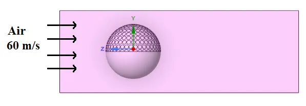
To begin with, an enclosure of suitable size is created in the Spaceclaim and the geometry is loaded to Ansys Mesh.

Mesh:

The Named selections are given and the Global mesh size is kept 0.004 m, for capturing the boundary layer effects, 8 inflation layers are provided with Growth rate of 1.2 and by smooth transition.

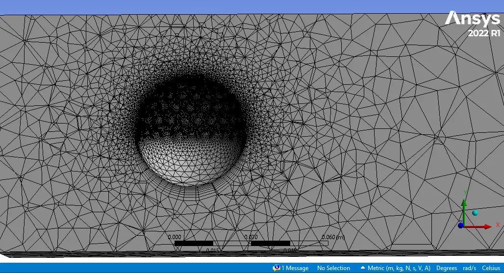
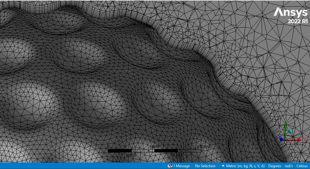
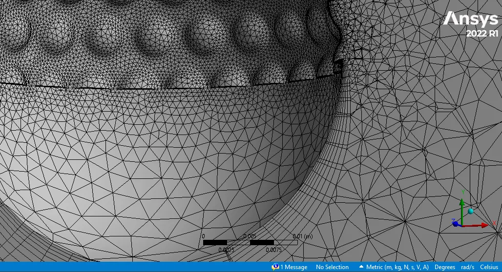
Since there is a change in curved boundaries as the upper surface has dimples and the lower surface does not have, there is a slight misalignment in the boundary layers for the lower surface.

Solver Settings:

The inlet is provided with Velocity inlet of 60 m/s and Outlet as Pressure Outlet at 1 atm.

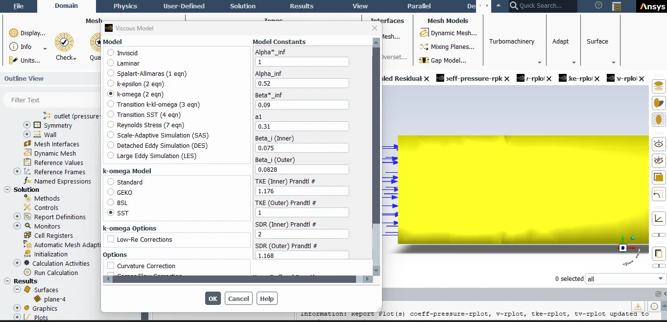
Since the flow has a low Reynolds Number, and will be wall bounded, the viscous model is set to k-omega SST.

The reference values are calculated from the inlet, with operating (Gauge) pressure as 0 pa.

With hybrid initialization, the case is ran for 500 iterations.

Countours and Plots:

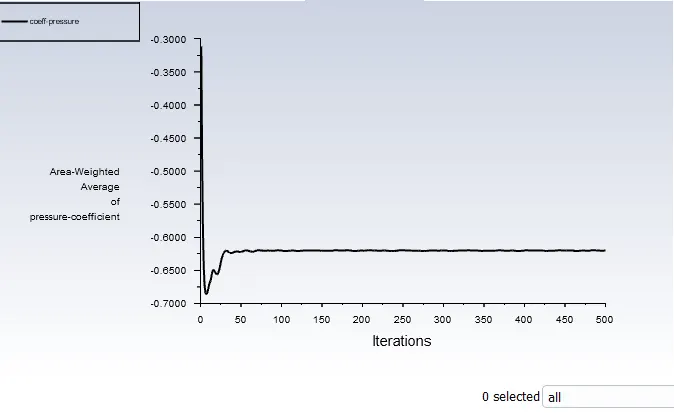
a. Variation in Coefficient of Pressure on ball

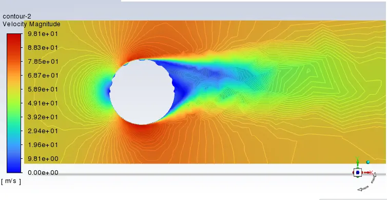
1. Countour of Velocity

Steady Behaviour:

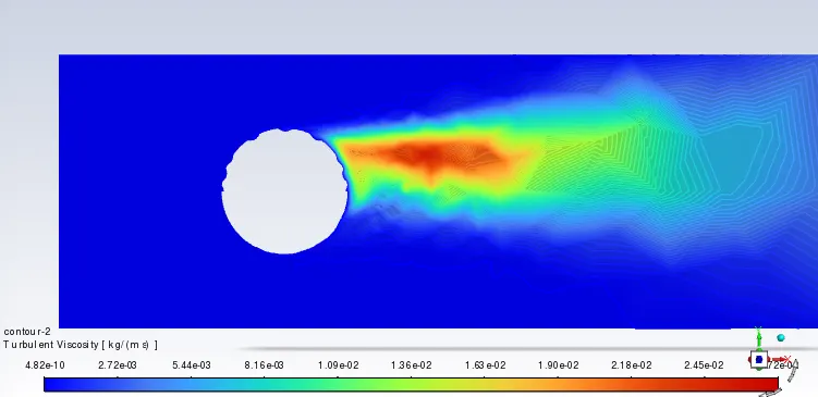
2. Countours of Viscosity

Steady Behaviour:

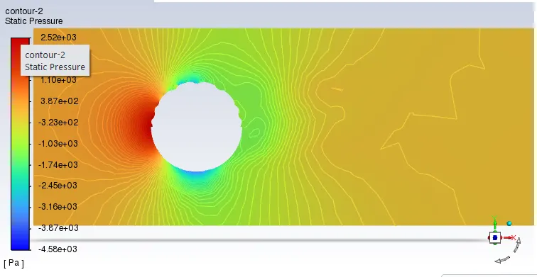
3. Countours of Static Pressure

Results and Discussion:

From the contour of pressure, a stagnation zone is formed at the frontal section and the Average value of Coefficient of Pressure being negative, around '-0.62', a lift is obtained for the current conditions. On the smooth side of the ball, a zone of low pressure is also observed.

The boundary layer is clearly visible on the upper side of the ball, which has dimples. This means that the momentum and energy exchange is more and the flow keeps detaching and reattaching the slotted surface while being in motion.

Based on the flow conditions around the ball, the ball will travel with about 60 m/s in direction opposite to air by clockwise direction.