Week 4.2: Project Transient simulation of flow over a throttle body

Advanced Aerodynamic Simulations using Converge Studio

Week 4.2 Project :- Transient state simulation of flow over a throttle body

Geometry setup and Pre-processing:

For the given project, a geometry of '.stl' file is loaded in Converge Studio. Since the imported geometry is not suitably captured by the CAD environment, few modifications are performed.

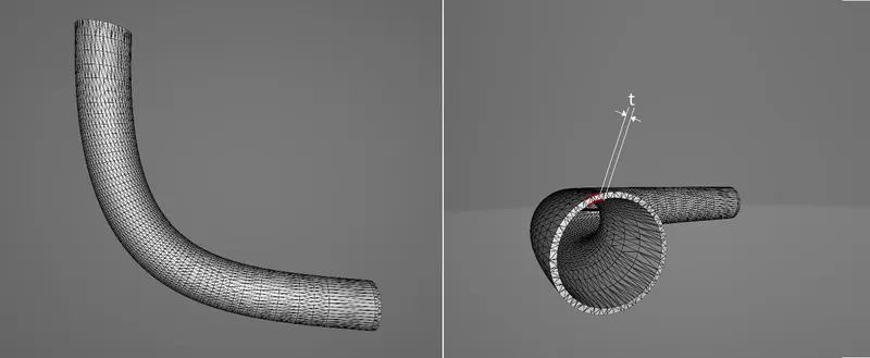
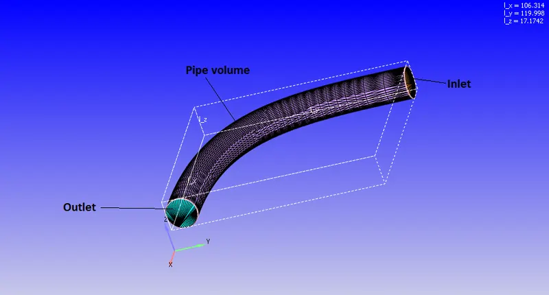
The aim here is to make internal flow analysis of the pipe. Here, the pipe has a wall thickness, which is not required and the internal flow volume is of importance. With that, the outer faces (width) of the geometry are removed and just a 2D surface is kept.

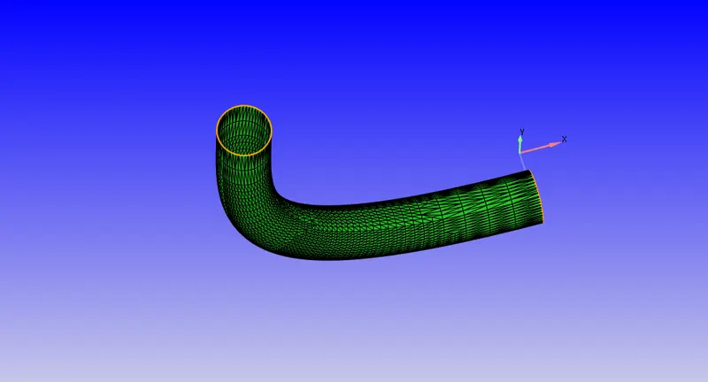
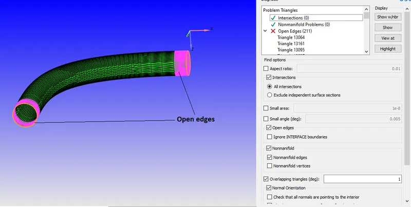
After removing the thickness, in order to make the geometry free of incomplete surfaces, the few open edges are removed and the open surfaces are sealed by providing patches at the circular openings, putting it simply, the open surface is covered by boundary fences at both ends.

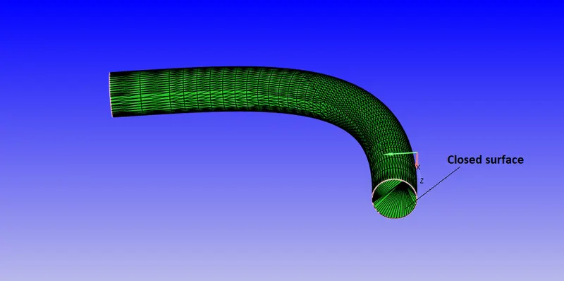
The image shown above represents the "Extracted Fluid Volume". In the next stage, the entire geometry consisting of triangles is categorized into inlet, outlet, pipe surface and the throttle body by creating different boundaries.

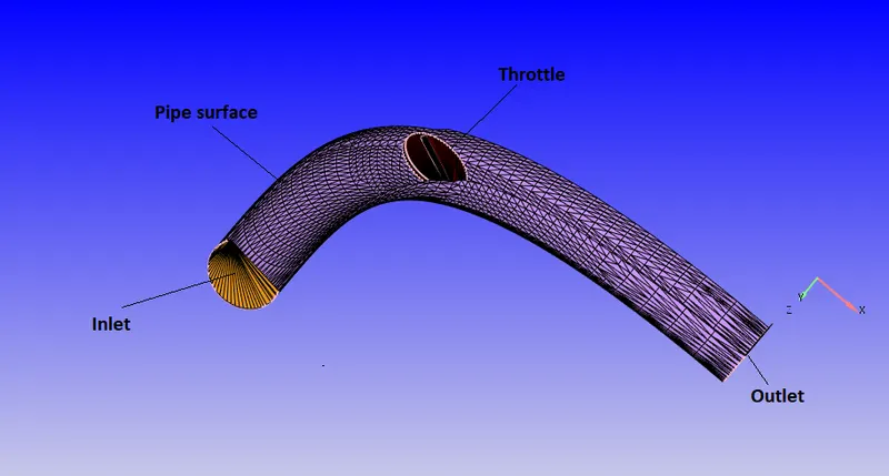
Nextly, the entire model is scaled down to a factor of 0.001. Here, the geometric dimensions will be reduced to an extent, however, the flow analysis will not be impacted.

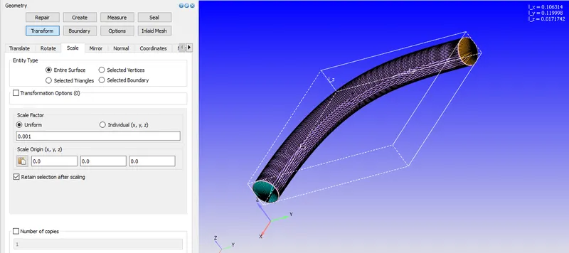
The geometry is free of any extra edges and is now ready for case setup.

Solver Settings:

In the Time-Based type of Transient state simulation, the fluid is chosen as 'Air', as mixture of N2 and O2 of 0.77 and 0.23 percent.

The Turbulent Prandtl number is a non-dimensional term defined as ratio between momentem eddy diffusivity and heat transfer eddy diffusivity. It is useful to solve heat transfer problem boundary layer flows. The summation of molecular and turbulent conductivity and diffusivity is taken into consideration when solving transport equations. With that, the turbulent Schmidt (Sc) and Prandtl number (Pr) are partially varying as presence of walls affect these values hence the default values taken near to 0.78 and 0.9 respectively.

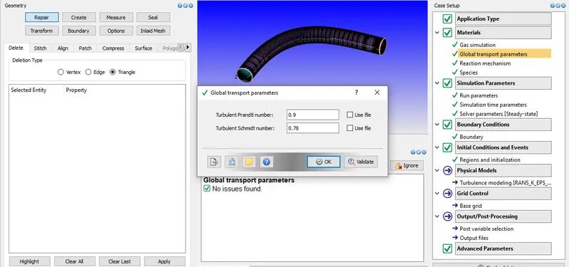
This default values is proved to be satisfactory for many reacting and non-reacting turbulent flows hence they can be used as some default approximations.

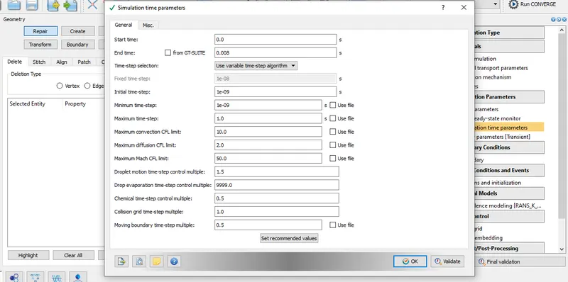
The case is set for full hydrodynamic and compressible flow and solver is preferred steady state solver. As the transient case setup is preffered, now its required to input the total flow time, which can be calculated as; Time = Characteristic length(scaled)/ Velocity, so with maximum distance of 0.2 with 180 m/s, the time is seconds is 0.001, and considering a little more value, the simulation duration will be 0.008 seconds. initial minimum time step of 1e-9 and maximum time step of 1 with maximum convection CFL limit of 0.5. The lesser the CFL number's value is, the slow will be the simulation and more accurate will it be. In addition the convective flux scheme is set as FVM and the Density based solver is used. These particular values of Convection CFL, Diffusion and Mach CFL number is related to the stabilty of the solution which Converge uses as default.

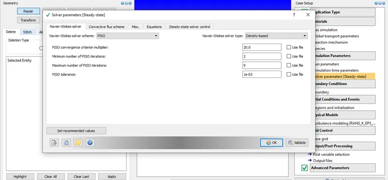
The solution scheme is set to PISO which is "Pressure Implicit with Splitting of Operator". The PISO algorithm with multiple time steps provides more stable solution, with lower time steps.

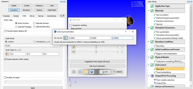
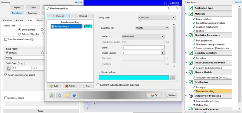
With regards to the grid size, the cell size is kept 0.0009 metres with total cell count of ~55000 cells. In addition to refine the regions at the internal boundaries, the Boundary type Permanant Fixed Embedding is employed at throttle surface, with scale of 2 and of total 4 layers

For Boundary conditions, the Inlet boundary is set to Total pressure inlet of 150000 Pa, with Zero Normal Gradient for Velocity Boundary condition, which means that all variables are set to a fixed value, and considering a variable is fully developed at the inflow region of the circular opening, so its variation with respect to space (`vecn`) is zero, i.e. `(dphi)/(dvecn)=0`.

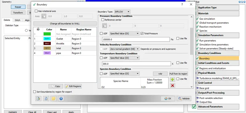
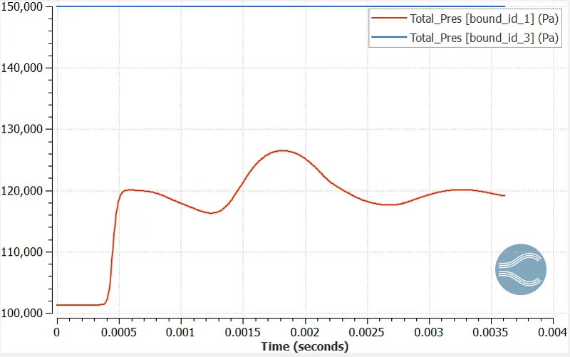
For outlet, the Pressure outlet is kept at 1 atm, i.e. 101325 Pa, at sea-level condition. By the pressure difference of ~48000 Pa, the value of velocity is around 280 m/s, setting up a compressible flow.

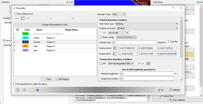
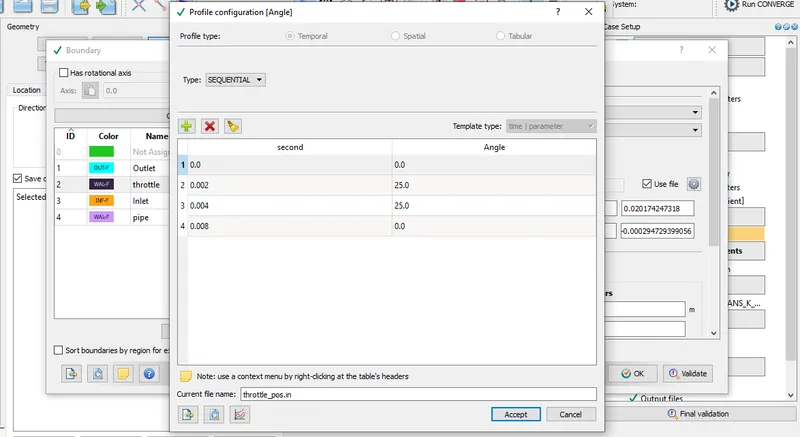
For the Throttle's boundary condition, as for an unsteady case, the Throttle has been kept moving by selecting motion type as 'Rotating' with moving surface. The arc centre and arc normal is measured using three vertices on the throttle. In the subsequent stage, the custom rotation rate is given as:

Rotation from 0 to 2 milliseconds will be 25 degrees, then from 2 to 4 milliseconds, the throttle will be at same position, i.e. at 25 degrees and following up by 8 milliseconds, the throttle will be at 0 degrees again.

The flow being viscous, the model is selected to RNG k-epsilon. In the standard k-Epsilon model, the eddy viscosity is determined by single turbulent length scale, however in reality all scales of motion contribute to turbulent diffusion so is this modified equation of Renormalised Group, (RNG k-epsilon) it accounts for different scales through changes in the production term.

After this the input files are exported to the case's setup folder and required executables along with license file are copied, and the case is analysed with 4 parallel processor in Cygwin. As the post processing of output files is done, the contours are viewed in Paraview and variation of parameters in Converge's line plot.

Post-Processing results:

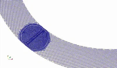
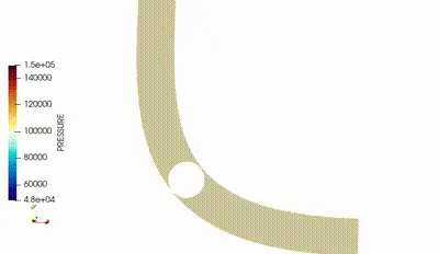
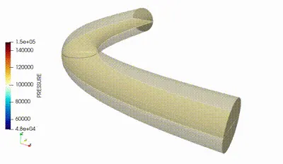
As the throttle is not steady here, the mesh will transform as well. The dynamic mesh of throttle is shown in below image.

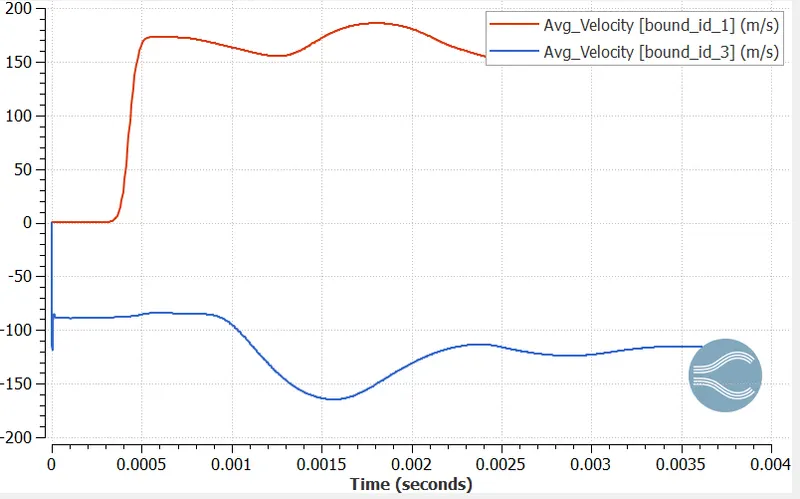
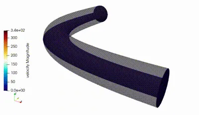
Variation in Velocity:

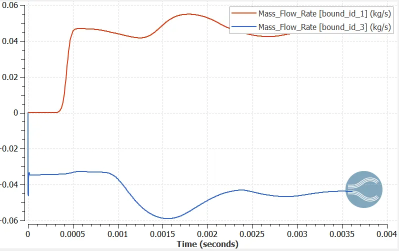
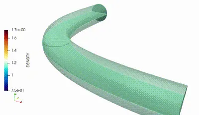
Variation in Mass flow rate:

Variation in Total Pressure:

Variation in Turbulent kinetic energy:

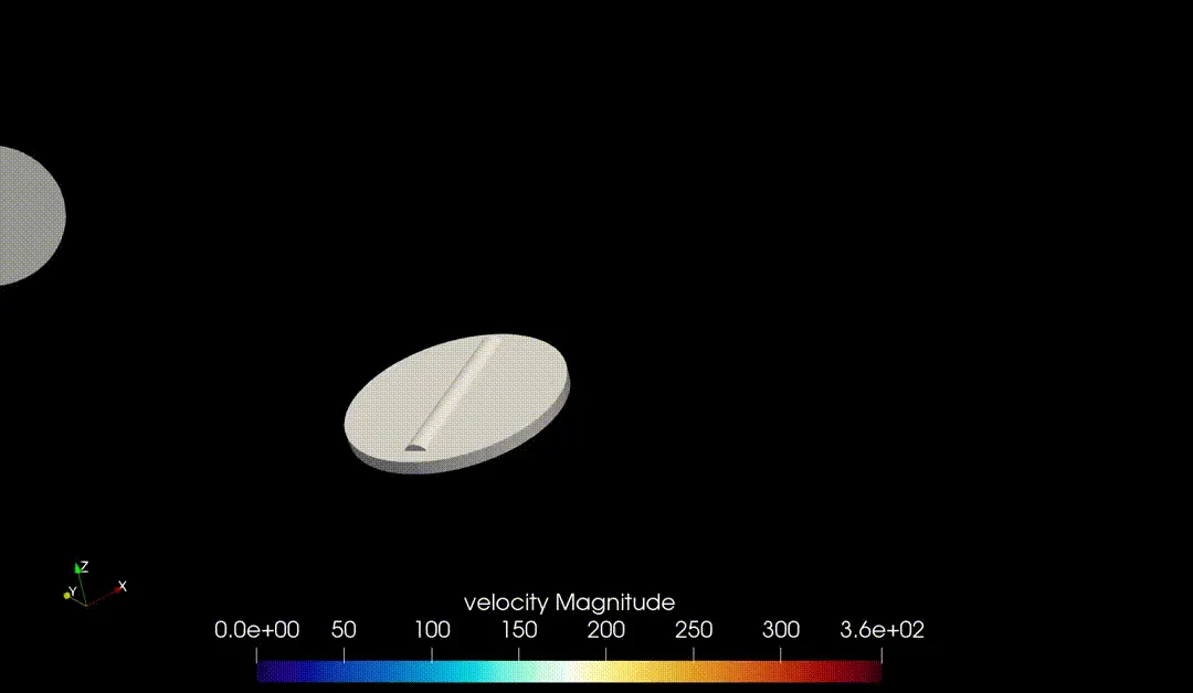
Variation in flow streamlines:

Conclusion:

As seen from the above plots of mass flow rate, the mass flux is conserved and the continuity equation is not violated. Secondly, there is fluctuation in pressure as the throttle valve is not stationary and so does the flow, however the outlet pressure is less near the end of the simulation time as compared to the inlet.

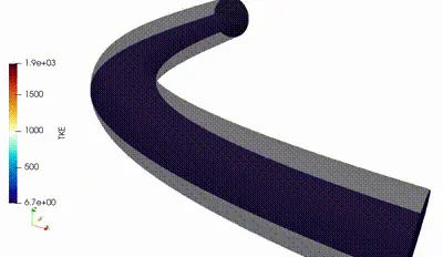
With regards to the turbulent kinetic energy, as soon as the throttle rotates, the eddies are formed with a reason of flow propogation is not completely smooth.

For the graph of velocity, at time 0.0015 second, a variation is observed in the velocity, which implies that a motion of throttle is taking place, and as a result, with a slight change in the flow passage, fluid is accelerated creating a little irregular pattern of flow at the other end of throttle. This change is also illustrated in the animation of streamline, when the throttle disc is rotated, there is curvature in flow streamlines at both adjacent side, with this the flow path is narrowed and thereby the streamlines (fluid) are at maximum velocity, but making a flow little disturbed because of movement of throttle itself.