Week 6: Conjugate Heat Transfer Simulation

Advanced Aerodynamic Simulations using Converge Studio

Week 6 Project :- Conjugate Heat Transfer Simulation

Conjugate Heat Transfer is referred when there is more than one way for the heat transfer to occur, like via conduction for solids and convection for fluid. Converge uses the Solid heat equation to deal with the Conjugate Heat Transfer problems, which is given as;

`Cp*rho*(delT)/(delt) = nabla*(knablaT) + S`

This represents the "Rate of change of temperature with respect to time in molecules is equal to the summation of heat flux as of convection and generation of a volumetric heat source".

Geometry setup and Pre-processing:

To begin with, instead of importing a CAD geometry in the studio, a 3-D cylindrical pipe with thickness is created, of 0.2 metres, and internal radius of 0.015 metre with an additional outer thickness of 0.05 metres.

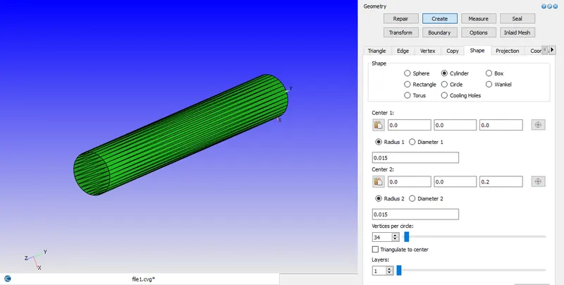
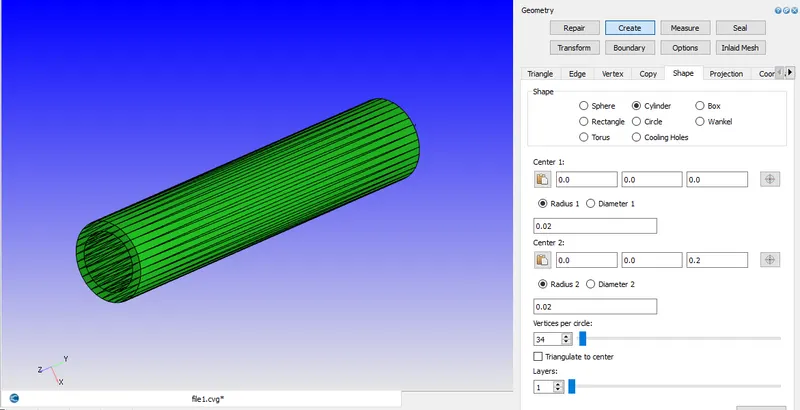
Since the created geometry has intersecting edges, the overlapping faces at frontal and backward area are removed.

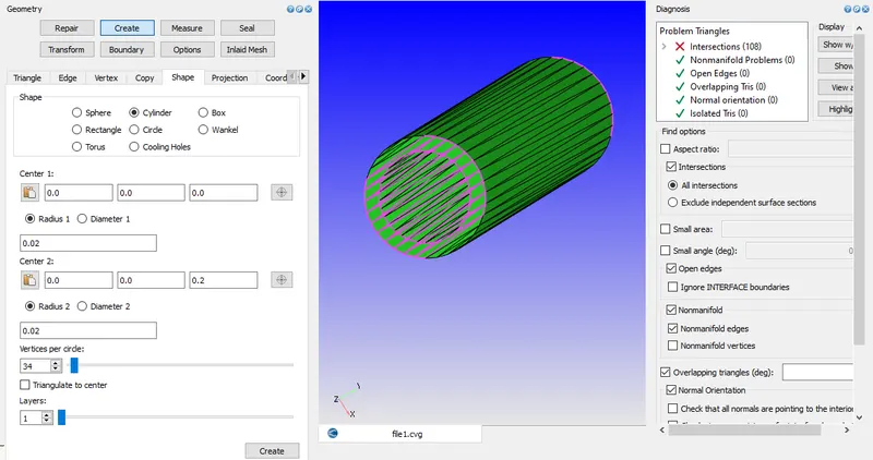
After removal of surface edges, the pipe is hollow and therefore filled regions need to be formed which acts as the solid thickness.

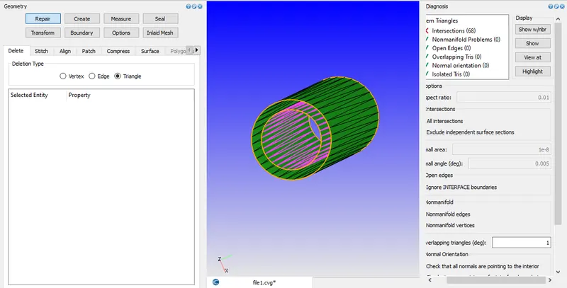
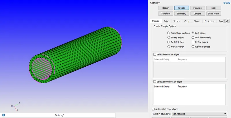
In order to settle this up, the open edges are lofted, by selecting the open edges of smaller and bigger radius.

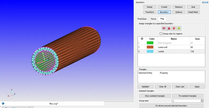
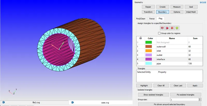
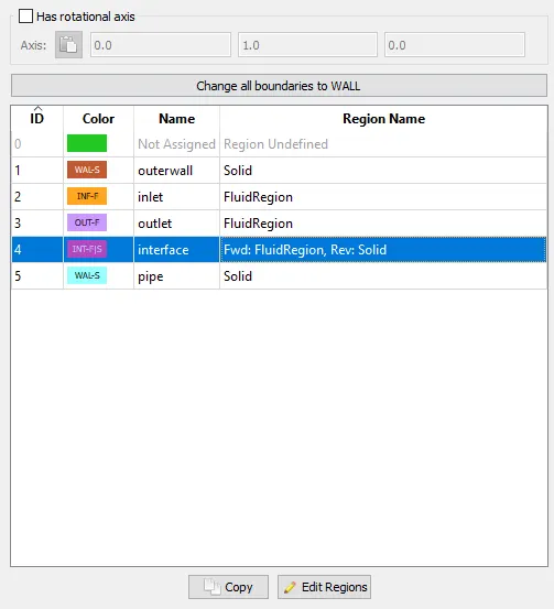
Subsequently, by creating the boundaries, the outermost surface is assigned as the outer wall and the solid of 0.05 metre as pipe.

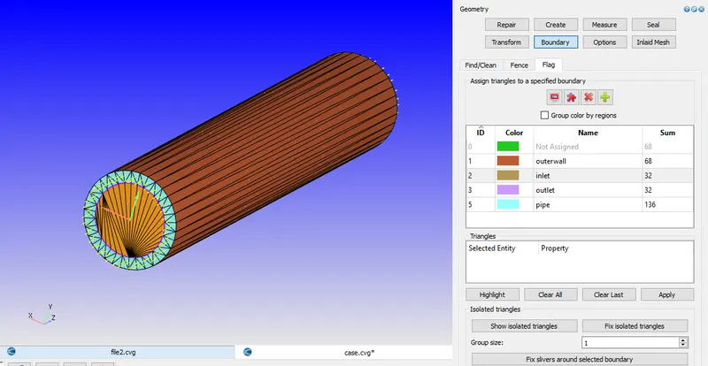
Finally, once checked whether the normals of the geometry are pointed in appropriate direction, the open face edges at frontal and back part are patched, making the hollow gap closed from the both ends, making possible to assign the boundaries as "Inlet" and "Outlet".

Right after this, if the diagnosis is ran, the an error of non-manifold edges is highlighted, which implies that the egde of one of the faces is shared by edged or faces of other faces.

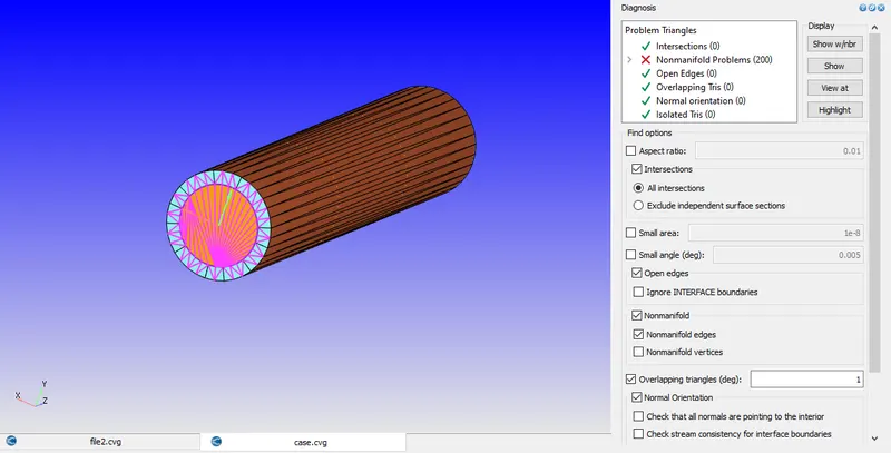
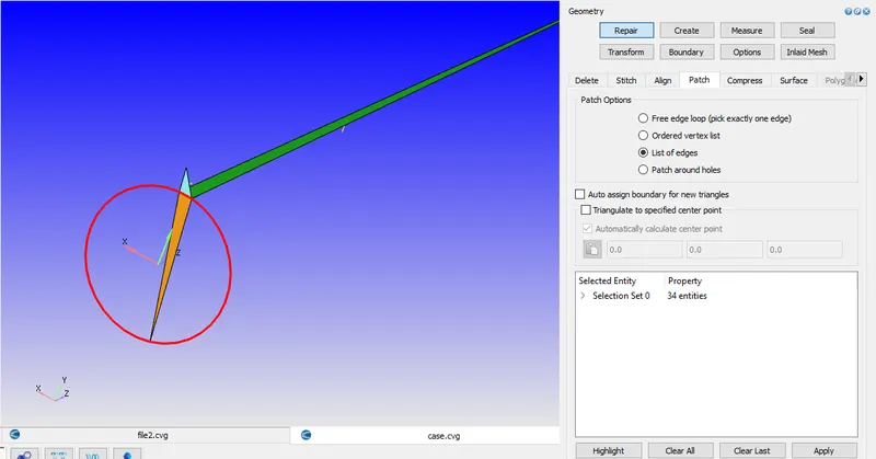
This error happens if the face which interacts with the fluid as well solid is not distinguished, so as its solution, the inner face is defined as "interface".

Solver Settings:

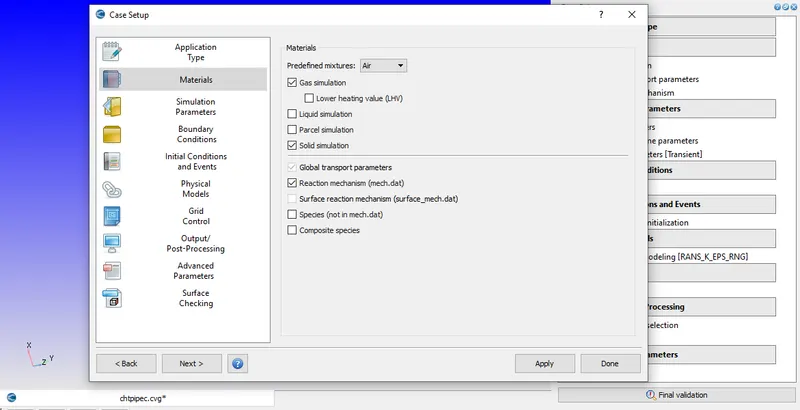
As the simulation deals with gas and solid as well, the case is preferred with solid and gas simulation.

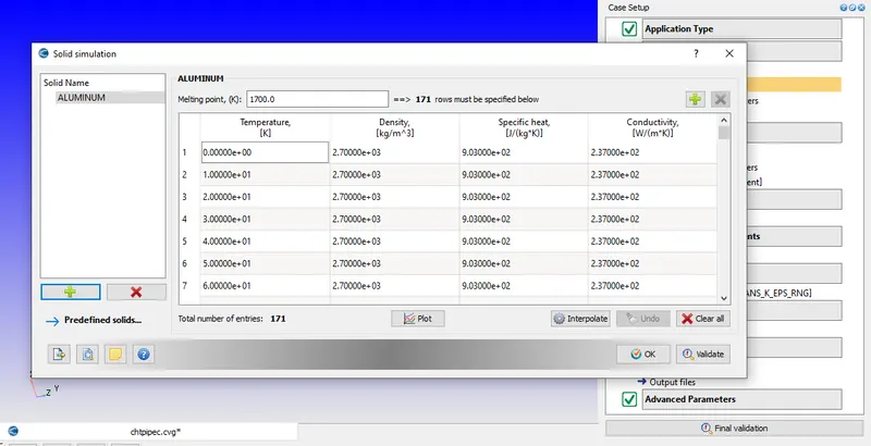
For the solid properties, the solid is assumed to be made of aluminium.

For the species, the mixture of oxygen and nitrogen is added for air and for solid, aluminium.

In the Time-Based type of Transient state simulation, the fluid is chosen as 'Air', as mixture of N2 and O2 of 0.77 and 0.23 percent.

Going with the case setup, the Redlich-Kwong equation is used as Equation of state as it is generally more accurate than the Ideal gas equation at temperatures above the critical temperatures, which is given as;

`p = ((R*T)/(V-b)) - ((a)/(sqrtT*V(V+b)))`,

where p is the Pressure

R is the Gas Constant

T is Temperature

V is Molar Volume (V/n)

a is a constant correction for attractive potential of molecules

b is a constant that corrects for volume

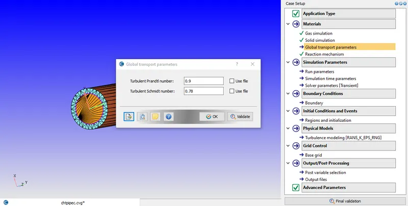
The Turbulent Prandtl number is a non-dimensional term defined as ratio between momentem eddy diffusivity and heat transfer eddy diffusivity. It is useful to solve heat transfer problem boundary layer flows. The summation of molecular and turbulent conductivity and diffusivity is taken into consideration when solving transport equations. With that, the turbulent Schmidt (Sc) and Prandtl number (Pr) are partially varying as presence of walls affect these values hence the default values taken near to 0.78 and 0.9 respectively. This default values is proved to be satisfactory for many reacting and non-reacting turbulent flows hence they can be used as some default approximations.

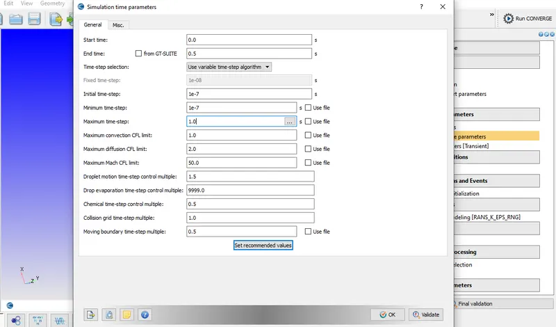
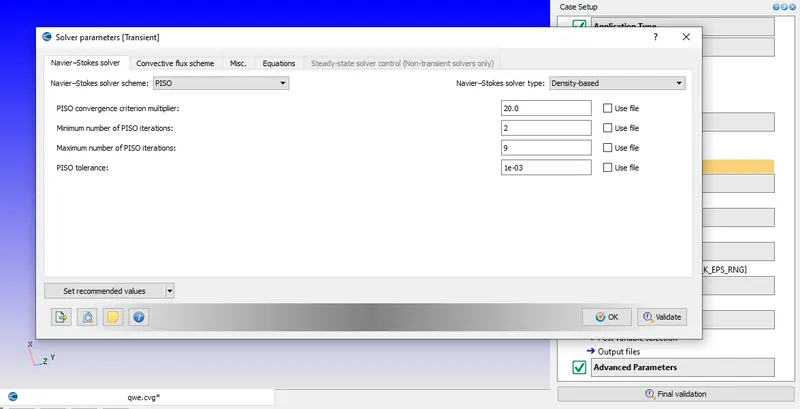
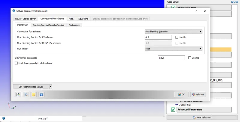
For the transient case, initial time is set to 0 seconds and end time to 0.5 seconds. minimum time step of 1e-7 and maximum time step of 1 with maximum convection CFL limit of 1. The lesser the CFL number's value is, the slow will be the simulation and more accurate will it be. In addition the convective flux scheme is set as FVM and the Density based solver is used. These particular values of Convection CFL, Diffusion and Mach CFL number is related to the stabilty of the solution which Converge uses as default.

Before defining the boundary conitions, two regions are created namely Fluid; which is at 300 K and 1 atm pressure with fluid as air and second as Solid with material as aluminium. Both the regions are having identical stream IDs.

Stream refers to a collection of connected groups having same material phase. This can be understood simply from the following chart;

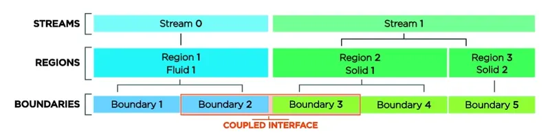
Even if the solid and the fluid regions are connected, they need to be differentiated, therefore providing a particular stream ID is important. The solver solves the PDEs while calculation, for fluids Navier-Stokes equations are solved and for solids, the solid heat conduction equation. So it is required to create a stream ID to let the Converge know that which equation is solved where.

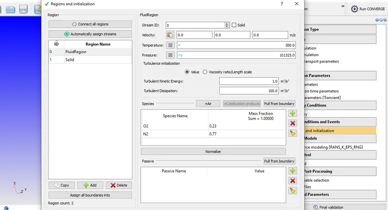
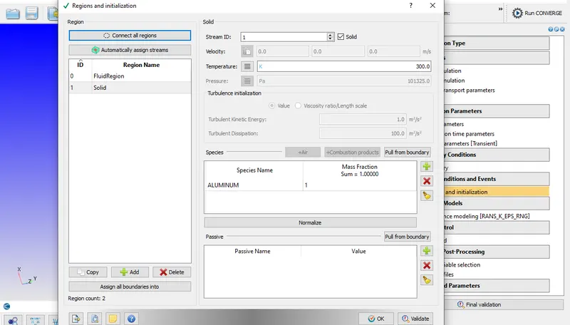
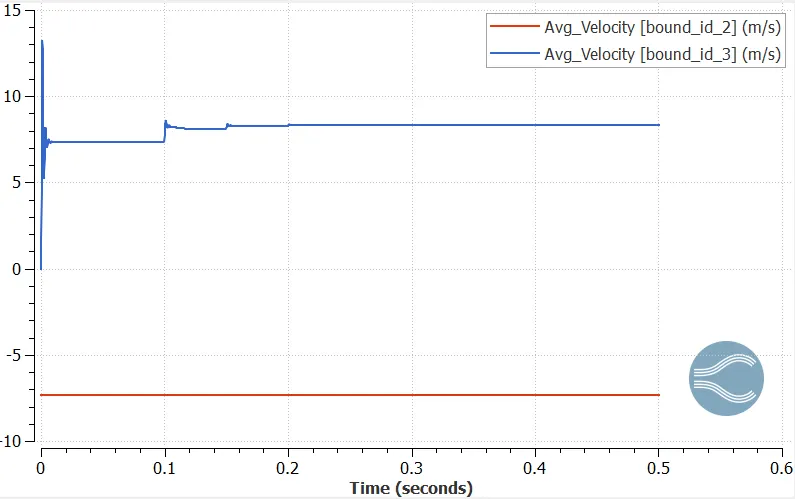
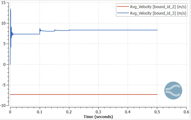
As far as the boundary conditions are concerned, the inlet is given as Inflow boundary (Dirichlet) condition. As the flow is to be simulated at Re 7000, with air density as 1.225 `(kg)/(m^3)`, and dynamic viscosity at sea-level as 1.79e-05 `(kg)/(ms)`, the fluid velocity comes out to be of 7.34 m/s. Since the geometry is aligned in Z-direction, the z component of velocity is given that value.

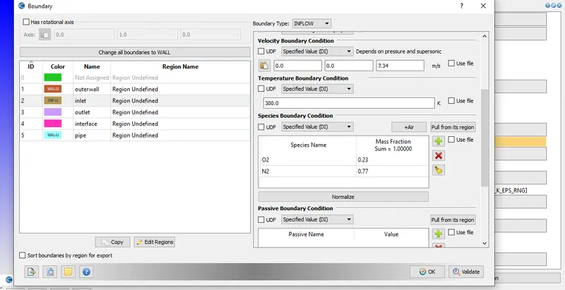
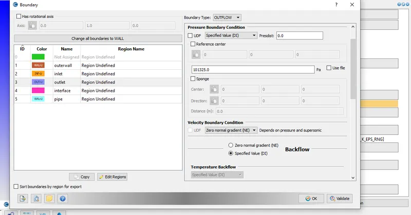
The outlet is given Outflow as atmospheric pressure of 1 atm.

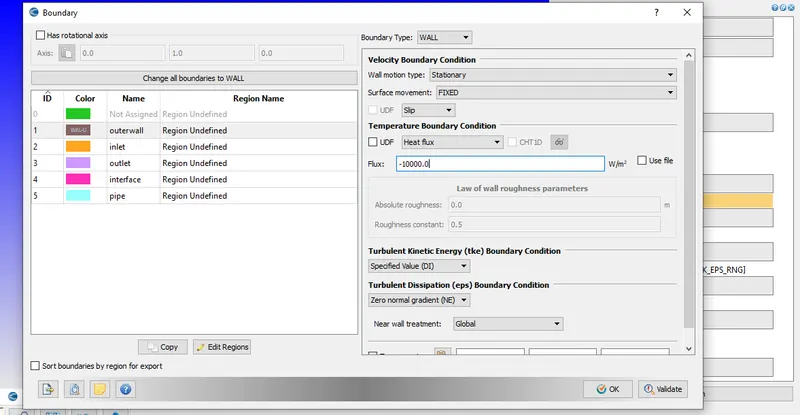
For the outer surface, type is given as Wall, here since the surface is solid, the Law of the wall condition is not applicable, so the stationary wall is given as Slip condition. With temperature setting as Heat Flux of -10000 `(W)/(m^2)`, implying that heat is ejected out of the surface.

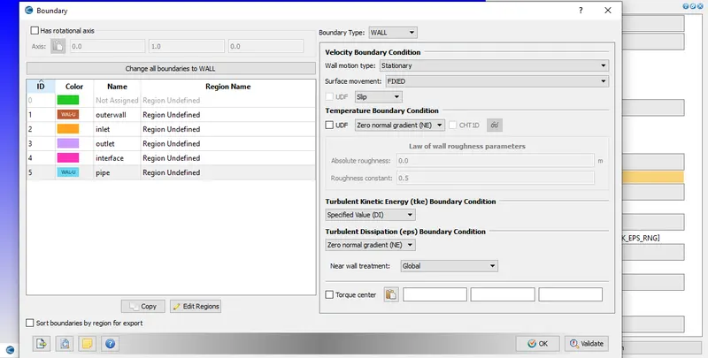
For the pipe, the boundary type is defined as Stationary wall with Slip condition, with Zero normal gradient, meaning that the that amount of 2D concentric surface is adiabetic and no heat transfer is taking place from that region.

Now, for the interface, where exist the contact between, solid and fluid, an Interface type of boundary condition is defined. This type boundaty will have a 2 sided definition, one where the normals are pointing inward, is called Forward Direction and other one pointing outward, is Reverse Direction. The Forward, the law of the wall is assigned as it points toward the fluid region, and for the Reverse side is alloted a Slip condition, pointing towards the solid.

At the interface boundary, the equations are coupled. From the solid to fluid, if the Contact resistance is kept zero, then the temperature profile, the heat transfer will be without any discontinuity else with any value of resistance, the temperature profile will not stay linear, i.e. there will be a drop in temperature values when propagated from solid to fluid via a resistance.

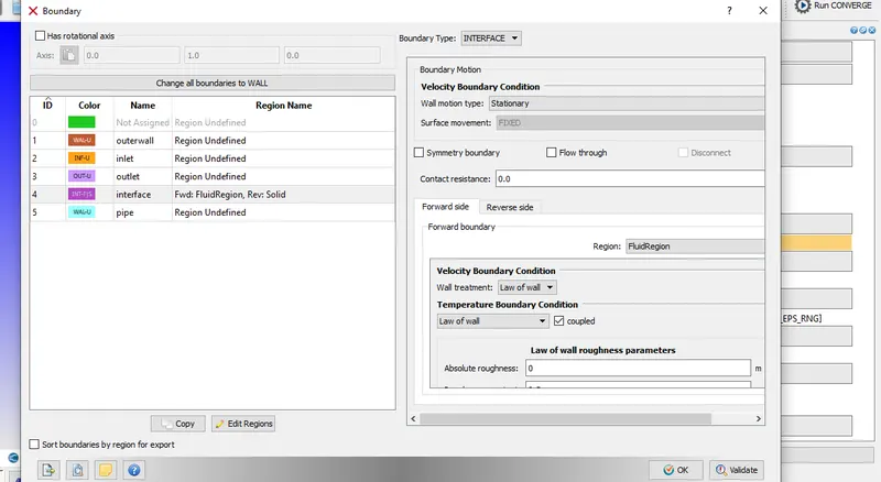
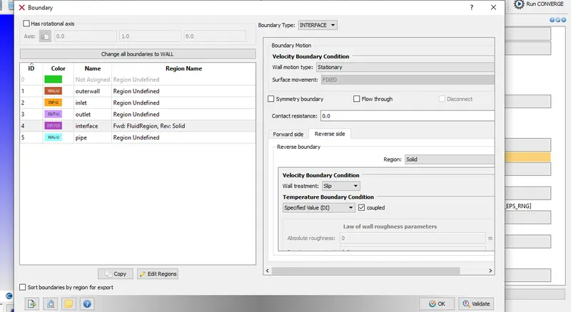
Lastly, all the boundaries are assigned with suitable regions.

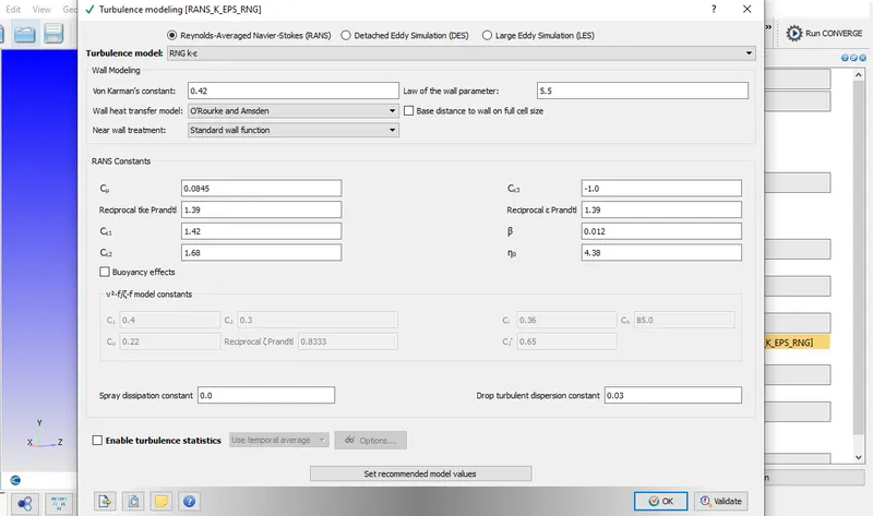
The flow being viscous, the model is selected to RNG k-epsilon. In the standard k-Epsilon model, the eddy viscosity is determined by single turbulent length scale, however in reality all scales of motion contribute to turbulent diffusion so is this modified equation of Renormalised Group, (RNG k-epsilon) it accounts for different scales through changes in the production term.

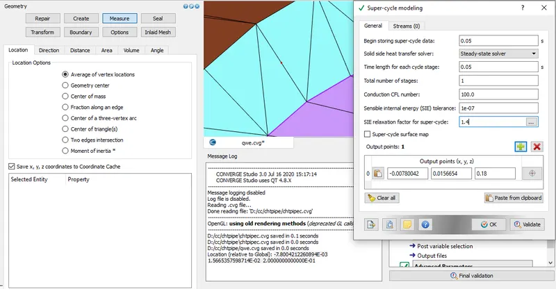
Super-cycling is enabled, with starting time of 0.05 seconds with same time length and the points on the pipe thickness are descreibed at which the temperature needs to be monitored, the z-direction value for space is kept 0.18, instead 0.2, as this particular point will then exist in the solid space to capture the data.

In the Transient approach, the case is solved from the start to end time, being divided the entire time scale into small time-steps and each time-step is solved very accurately, but it consumes large amount of time, as calculating the heat transfer process in solids can be time consuming unlike the flow thru a pipe, however, in the Steady state approach the chronological behaviour of the process is not given that importance, and thus giving final temperature distribution rapidly in cases where fluid flow and heat transfer process has a steady pattern.

In Super-cycling, the flow calculation is done completely with transient approach and by regular intervals steady-state calculation is conducted for the solid, hence delivering results more quickly as compared to the transient method. Initially, the solver solves fluid and solid part transiently for certain time, thereafter the both parts' temperature values are averaged. Nextly, the fluid solver is kept frozen and simultaneously the solid part is solved via steady state approach, thereafter tne fluid solver is unfreezed and both parts are solved with respect to time again and the same cycle keeps on repeating.

"Super-cycling ensures the final temperature values are accurate because the gas part is calculated time-sensitively".

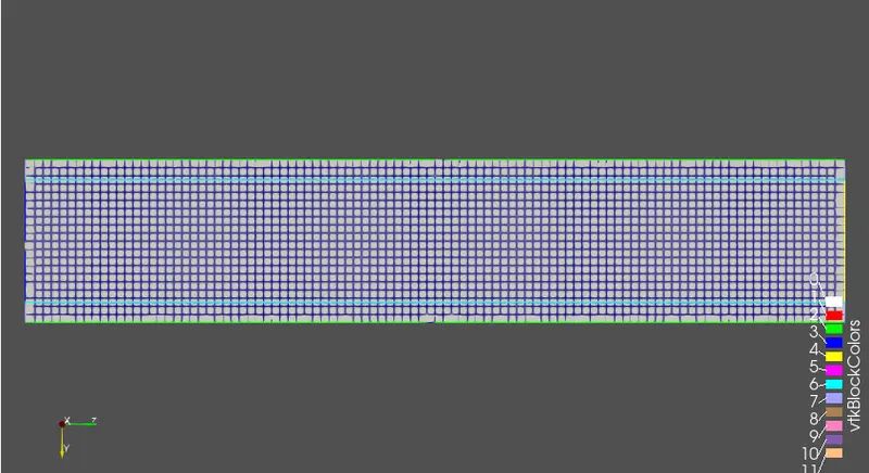
The base grid size is kept 0.004 metres with total approximate 5638 cells and time interval for writing the output data is kept 0.01 seconds.

The setup is ran for 3 different mesh sizes by varying the values of Super-Cycling.

After this the input files are exported to the case's setup folder and required executables along with license file are copied, and the case is analysed with 4 parallel processor in Cygwin. As the post processing of output files is done, the contours are viewed in Paraview and variation of parameters in Converge's line plot.

Post-Processing results:

Plots of mesh size 0.004 m, and super-cycling 0.05:

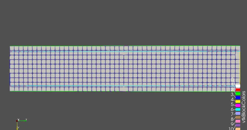
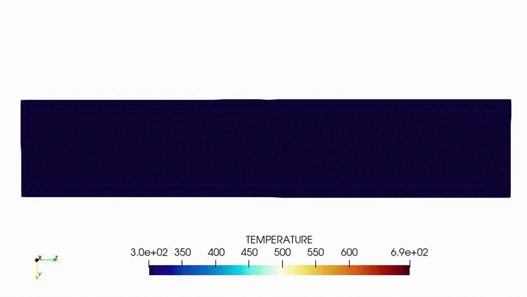
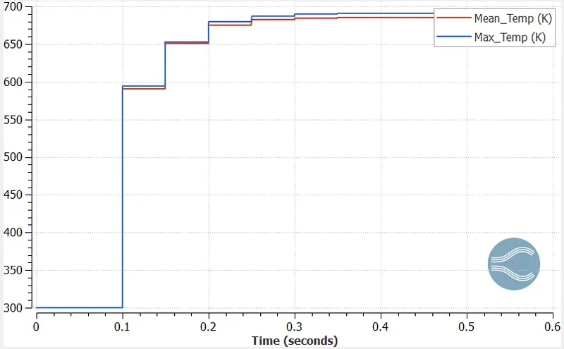
Variation in solid temperature:

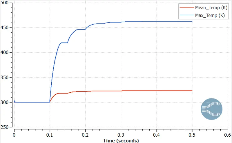
Variation in fluid temperature:

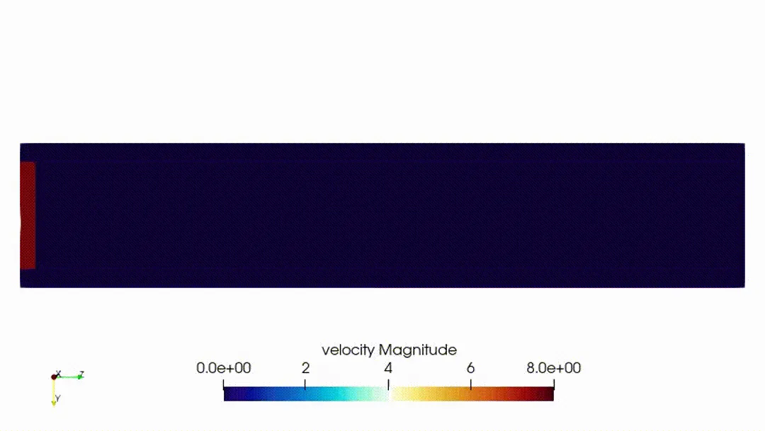
Variation in fluid velocity:

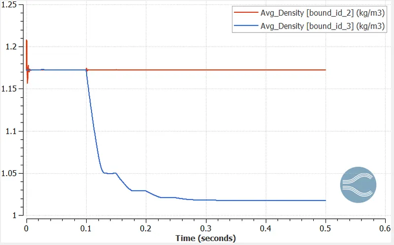
Variation in fluid density:

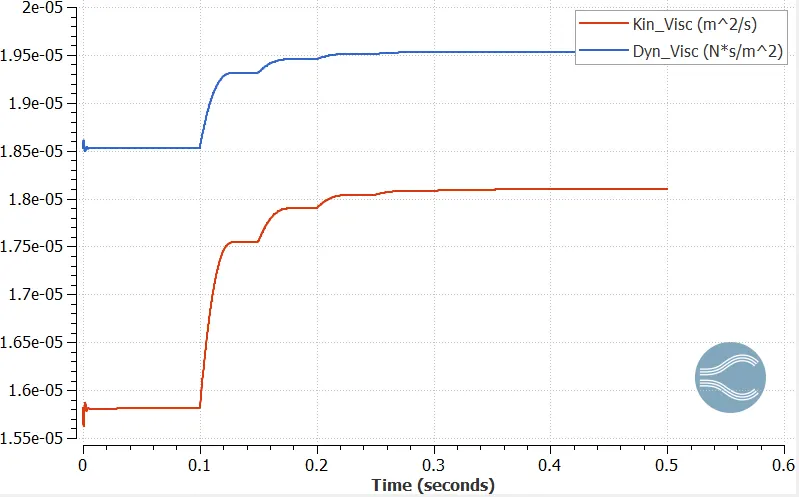
Variation in fluid viscosities:

Plots of mesh size 0.0025 m, and super-cycling 0.05:

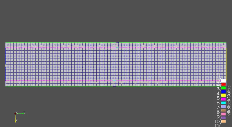
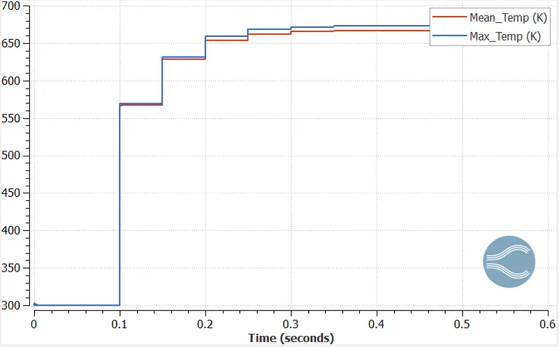
Variation in solid temperature:

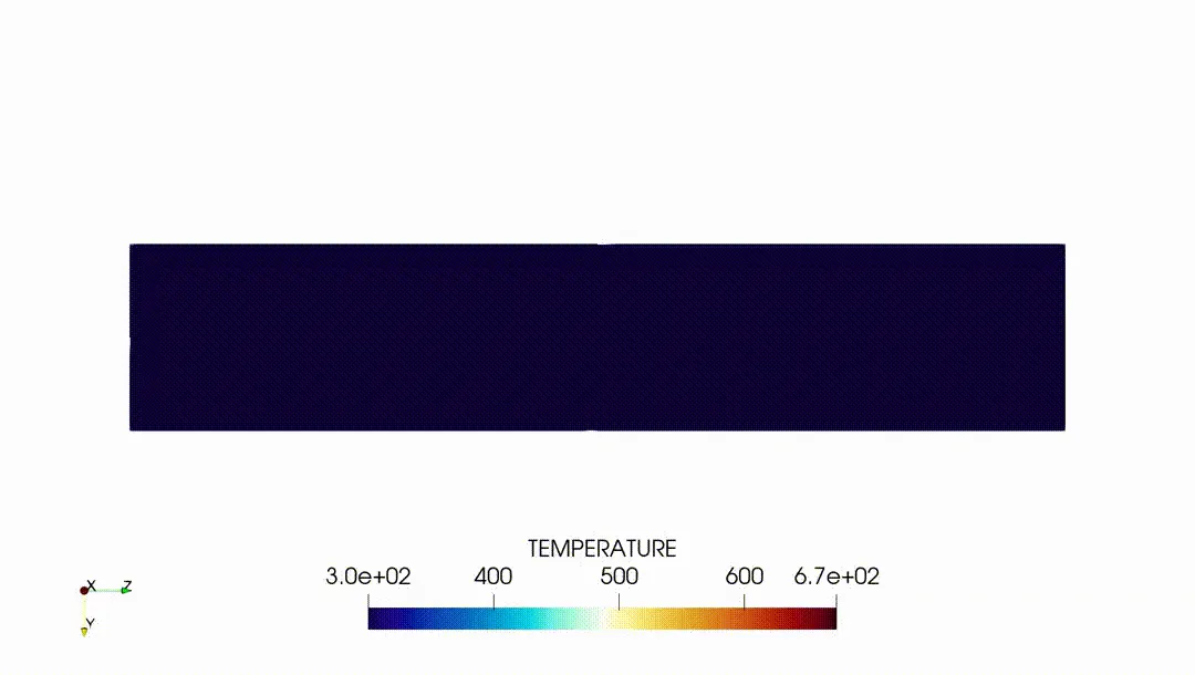
Variation in fluid temperature:

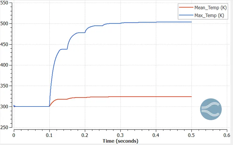
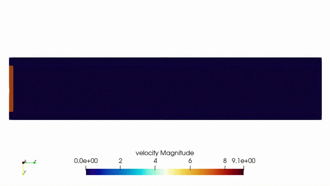
Variation in fluid velocity:

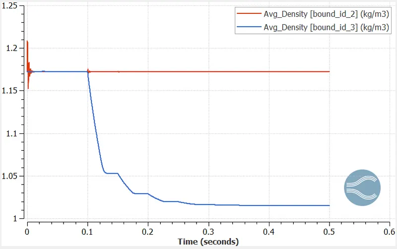
Variation in fluid density:

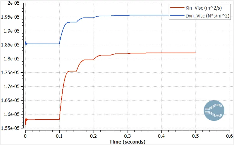
Variation in fluid viscosities:

Plots of mesh size 0.00199 m, and super-cycling 0.05:

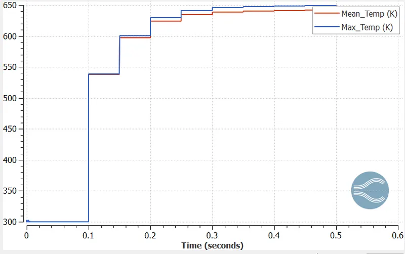
Variation in solid temperature:

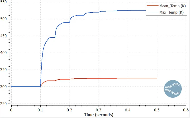
Variation in fluid temperature:

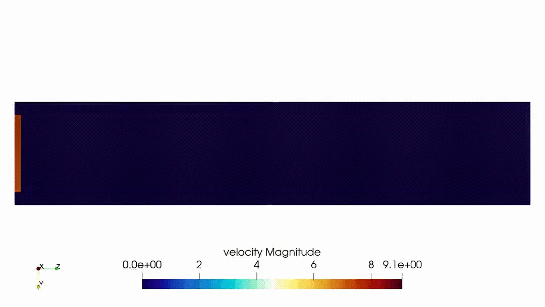
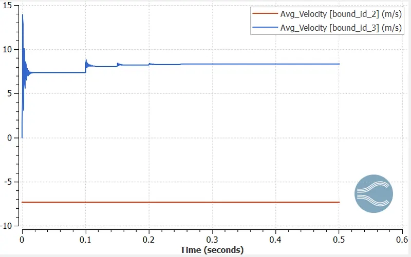
Variation in fluid velocity:

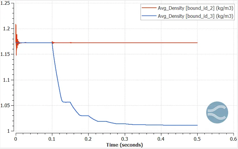
Variation in fluid density:

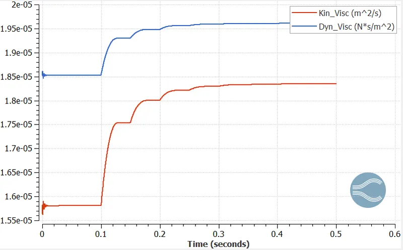
Variation in fluid viscosities:

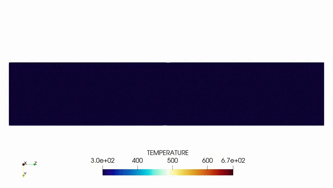
Variation in temperature distribution of pipe:

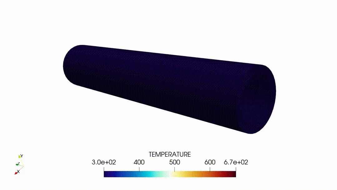
With inlet v=7.34m/s and temperature 300 K, following is noted from the graphical plots attached above:

Sr. No.	Mesh Size (metre)	Total cells	Outlet Fluid Velocity (m/s)	Mean Outlet Temperature of Fluid (K)	Max. Outlet Temperature of Fluid (K)	Mean Outlet Temperature of Solid (K)	Max. Outlet Temperature of Solid (K)
1.	0.004	5368	8.4	323	462	685	690
2.	0.0025	21991	8.34	323	503	666.3	673.8
3.	0.00199	43602	8.33	324.9	524.9	641.1	648.8

Effect of Super-cycling:

Sr, No.	Mesh size	Cells	Super- Cycling value	Simulation time (min.)
1.	0.00199 m	43602	0.05	65
2.	0.00199 m	43602	0.03	58.26
3.	0.00199 m	43602	0.01	54.1

Conclusion:

As seen from the graph of variation in solid temperature, the initial value is 300 K at 0 second, and right after 0.1 second, a drastic jump in the temperature is seen making the solid temperature near about 600 K because of Super-cycling. The heat capacitance of solid is much more as compared to those of fluid, hence without super-cycling, it could take a lot more time for the solid to reach that temperature. Thereafter, with the intervals of 0.1 second, slight small increments are seen gradually converging to a specific value of temperture. This was with the case of the aluminium, having a fixed specific heat capacity, based with variation of the materials, super-cycling can be useful in predicting the heat transfer in solids quite effectively.

Secondly, the initial fluid temperature is 323 K and after certain time, the temperature rises, thereby decreasing the viscosity of fluid along with the density. With regards to the mesh quality, the data is captured better when the element quality is fine. This can be well understood from the outlet temperature values for fluid as well as solid. As the mesh gets better, the average and maximum temperature are better predicted.

Furthermore, with the variation in super-cycling values, keeping the mesh size same, the simulation time is reduced. Lower the super-cycling values, values converge more quickly.