Week 4 - Genetic Algorithm

AIM :-

To write a program in MATLAB to optimise a stalagmite function through genetic algorithm and also to find the global maxima of the function.

THEORY :-

Optimisation is the process of selecting the best element from a set of available alternatives. It consists of maximizing or minimising a function by choosing the input values from a set and computes the values of the solution. In optimisation there are two methods,

• Deterministic Model: In deterministic models, the output of the model is fully determined by the parameter values and the initial conditions.
• Stochastic Model: Stochastic models possess some inherent randomness. The same set of parameter values and initial conditions will lead to an ensemble of different outputs.

What is maxima and minima,

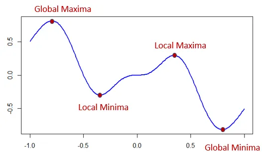
Local maxima: It is the point where the height of the function at a particular location is greater than the height in an interval.

Local minima: It is the point where the height of the function at a particular location is lesser than the height in an interval.

Global maxima or minima: It is the maxima or minima over the entire function.

In a function there can be multiple local maxima or minima over the function but only one global maxima and minima over the function.

A genetic algorithm an optimisation tool which is based on Charles Darwin's theory of Natural Selection. Natural selection is based on the survival of the fittest where the parents with better fitness will have offsprings which inherits the trait of their parents and improve their chances of survivability. This process keeps happening until the fittest generation i found.

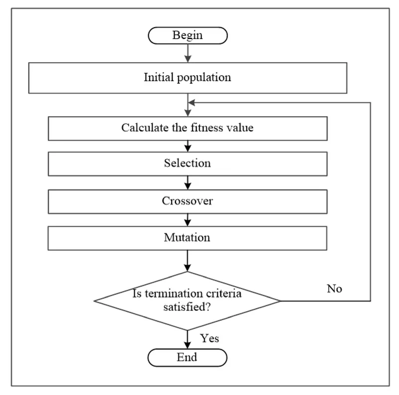
There are 5 processes involved in genetic algorithm,

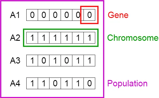
Initial Population: The process begins with a set of individuals called as population. Each individual is a solution of the given problem. An individual is characterised by a set of parameters called genes. These are combined as a set to get a chromosome or a solution.

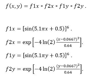
Fitness Function: This function determines how fit a solution is. It gives a fitness score to each solution and the probability of a particular individual being selected in the population for reproduction is based on the fitness score. The function used for the program is given below,

Selection: This process is done to select the fittest solutions and pass their variables to the next generation. Two pair of solutions are selected based on their fitness scores and the solution with the higher fitness have a better chance of reproduction.

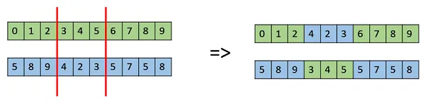
Crossover: In this process, for each pair of solution to be mated, a crossover point is selected at random among the variables. The offsprings are created by exchanging the variables of the solution amongst themselves and the new offsprings are added to the population.

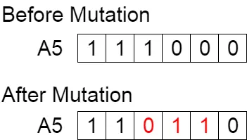
Mutation: In certain offsprings, the variables undergo mutation for those having a low random probability. Here the variables get flipped inside the solution. This process is done to maintain diversity within the population and prevent premature convergance.

Termination: The algorithm terminates if the population has converged. Then it is said that the genetic algorithm has provided a set of solutions to the problem.

Genetic Algorithm Syntax in MATLAB :-

The standard syntax for genetic algorithm is given as x = ga (fun,nvars); . This syntax finds a local unconstrained minimum x to the objective function fun, where nvars is the dimensional number of variables of the function.

The syntax of genetic algorithm with bounded conditions is given as x = ga (fun,nvars, A, b, Aeq, beq, lb, ub); . This defines a set of lower and upper bounds on the design variables x, so that a solution is found in the range lb ≤ x ≤ ub.

The syntax to increase the number of iterations of the genetic algorithm is given as x = ga (fun,nvars, A, b, Aeq, beq, lb, ub, nonlcon, Intcon, options); .

MATLAB PROGRAM :-

First a program to define the fitness function is written.

% Stalagmite function
function [f] = stalagmite(input_vector)
x = input_vector(1);
y = input_vector(2);

% Defining the x values
f1x = (sin(5.1*pi*x+0.5)).^6;
f2x = exp((-4*log(2)*((x-0.0667).^2)/0.64));

% Defining the y values
f1y = (sin(5.1*pi*y+0.5)).^6;
f2y = exp((-4*log(2)*((y-0.0667).^2)/0.64));

[f] = -(f1x*f2x*f1y*f2y);
end

Once the code for defining the function is written, the program for the three cases is given below.

1. Study-1: Statistical Behaviour.

% Genetic algorithm Statistical behaviour
clear all
close all
clc

% Defining the search space
x = linspace(0,0.6,150);
y = linspace(0,0.6,150);
num_cases = 50;           % To run the command 50 times.

% Creating a 2D mesh
[xx,yy] = meshgrid(x,y);

% Evaluating the stalagmite function
for i = 1:length(xx)
    for j = 1:length(yy)
        input_vector(1) = xx(i,j);
        input_vector(2) = yy(i,j);
        f(i,j) = stalagmite(input_vector);
    end
end

% Calling the Genetic Algorithm
tic
for i = 1:num_cases
    [inputs,fopt(i)] = ga(@stalagmite,2);
    xopt(i) = inputs(1);
    yopt(i) = inputs(2);
end
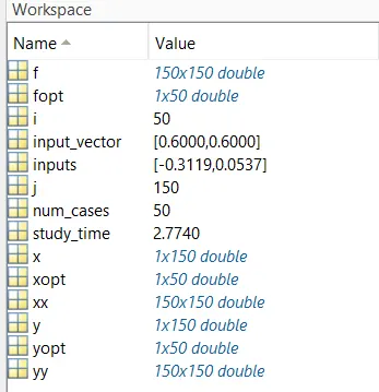
study_time = toc

% Plotting the function
figure(1)
subplot(2,1,1)
hold on
surfc(x,y,-f)
shading interp
plot3(xopt,yopt,-fopt,'marker','o','markersize',5,'markerfacecolor','r')
title('Unbounded inputs')
subplot(2,1,2)
plot(-fopt)
xlabel('Iterations')
ylabel('Function maximum')

2. Study-2: Bounded Conditions.

% Genetic algorithm Bounded Conditions
clear all
close all
clc

% Defining the search space
x = linspace(0,0.6,150);
y = linspace(0,0.6,150);
num_cases = 50;           % To run the command 50 times.

% Creating a 2D mesh
[xx,yy] = meshgrid(x,y);

% Evaluating the stalagmite function
for i = 1:length(xx)
    for j = 1:length(yy)
        input_vector(1) = xx(i,j);
        input_vector(2) = yy(i,j);
        f(i,j) = stalagmite(input_vector);
    end
end

% Calling the Genetic Algorithm
tic
for i = 1:num_cases
    [inputs,fopt(i)] = ga(@stalagmite,2,[],[],[],[],[0;0],[1;1]);
    xopt(i) = inputs(1);
    yopt(i) = inputs(2);
end
study_time = toc

% Plotting the function
figure(2)
subplot(2,1,1)
hold on
surfc(x,y,-f)
shading interp
plot3(xopt,yopt,-fopt,'marker','o','markersize',5,'markerfacecolor','r')
title('Bounded inputs')
subplot(2,1,2)
plot(-fopt)
xlabel('Iterations')
ylabel('Function maximum')

3. Study-3: Increasing the Iterations.

% Genetic algorithm, increasing the iterations
clear all
close all
clc

% Defining the search space
x = linspace(0,0.6,150);
y = linspace(0,0.6,150);
num_cases = 50;           % To run the command 50 times.

% Creating a 2D mesh
[xx,yy] = meshgrid(x,y);

% Evaluating the stalagmite function
for i = 1:length(xx)
    for j = 1:length(yy)
        input_vector(1) = xx(i,j);
        input_vector(2) = yy(i,j);
        f(i,j) = stalagmite(input_vector);
    end
end

options = optimoptions('ga');
options = optimoptions(options,'PopulationSize',170);

% Calling the Genetic Algorithm
tic
for i = 1:num_cases
    [inputs,fopt(i)] = ga(@stalagmite,2,[],[],[],[],[0;0],[1;1],[],[],options);
    xopt(i) = inputs(1);
    yopt(i) = inputs(2);
end
study_time = toc

% Plotting the function
figure(3)
subplot(2,1,1)
hold on
surfc(x,y,-f)
shading interp
plot3(xopt,yopt,-fopt,'marker','o','markersize',5,'markerfacecolor','r')
title('Increasing iterations')
subplot(2,1,2)
plot(-fopt)
xlabel('Iterations')
ylabel('Function maximum')

EXPLANATION OF THE PROGRAM :-

The general structure of the code is the same for all the three cases, with the only different being the genetic algorithm syntax ga for each case.

• We first start with defining the search space x and y as linear spaced arrays.
• A command num_cases is added to run the iteration 50 times.
• The search space is then converted to a 2 Dimensional array using the command meshgrid.
• In order to call the function to plot the stalagmite, a for loop is used and the values are stored in an array called input_vector.
• The function is defined as a negative function because, the ga solver only calculates the minima. By inverting the function we will be able to plot the stalagmite to calculate the maxima.

For Study-1,

• In this case the conditions are unbound and the ga function takes the iterations at random and solves them.
• The ga is called by using a for loop and the variable fopt is used to get the optimal function. The optimal values of x and y are stored as inputs(1) and inputs(2) respectively.
• To get the time taken to solve the iterations, we use the tic toc command.
• To plot the stalagmite function a subplot is created and the surf command is used to get a 3 Dimensional graph.
• The shading interp command is used to shade the graph and remove the grid lines that are formed by default with the surface plot.
• To determine the maxima within the stalagmite plot, the plot3 command is used to create a line plot which plots the optimum values of x, y and f.
• In order to understand the maxima at each iteration more clearly, we create another subplot within the figure to plot the optimal function obtained.

For Study-2,

• The same steps are followed as in study 1 with the main change being a different syntax used to call the ga.
• In this case we define some boundaries to plot the maxima. We use the syntax [inputs,fopt(i)] = ga(@stalagmite,2,[],[],[],[],[0;0],[1;1]); . Here [0;0] is the lower bound of the function and [1;1] is the upper bound of the function. A null matrix [] is used to fill in the empty spaces to complete the syntax.

For Study-3,

• In this study we increase the number of iterations the ga function has to solve.
• This is done by using the options command which is used to define the population size.
• Once the population size is defined, the ga function is called using the syntax [inputs,fopt(i)] = ga(@stalagmite,2,[],[],[],[],[0;0],[1;1],[],[],options); . The additional input along with defining the boundaries is options which defines the population size of the function.

RESULTS :-

The plots of each case are obtained and shown below,

1. Study-1: Statistical Behavior.

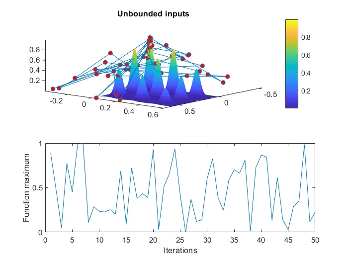
In this case we can see that the maxima obtained is all over the place, this solution is not optimal in order to find the global maxima.

2. Study-2: Bounded Conditions.

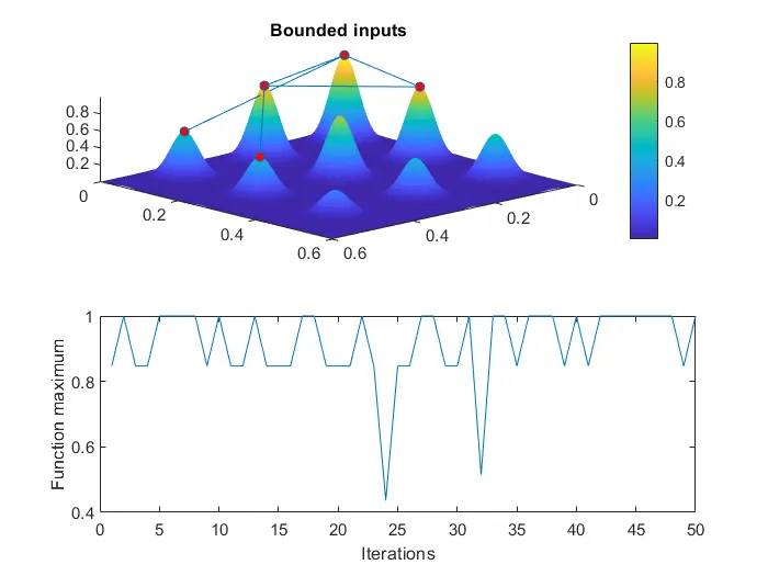
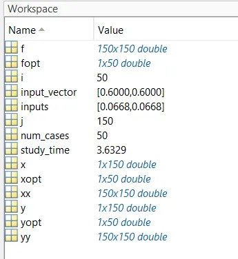
Here by defining boundaries for the varies we are able to get a clearer output to obtain the local maxima. But it is still not accurate enough to obtain the global maxima.

Study-3: Increasing the iterations.

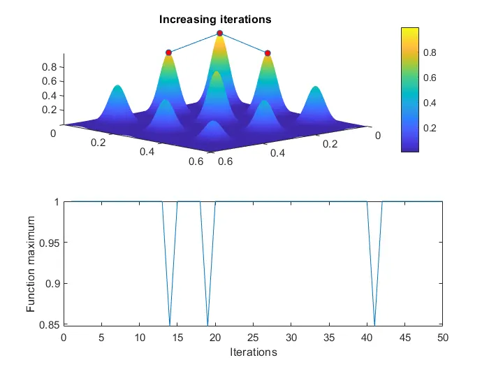
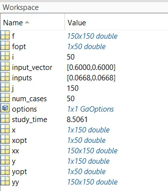
In this case along with the boundary conditions we also define the population size. In doing so we get a very clear plot that gives us the global maxima of the given function.

CONCLUSION :-

• Using MATLAB we were able to plot a stalagmite function using genetic algorithm.
• We were able to plot the function for three different cases.
• We were able to calculate the global maxima of the given function.