Final Project: Electric Rickshaw modelling

AIM :-

To create a MATLAB model of an electric rickshaw based on the following parameters.

• Rear wheels to be driven by a permanent magnet brushed type DC motor.
• The efficiency points of the motor and controller should be assumed.
• Create an excel sheet of the input and assumed data.

The following results must be obtained from any three driving cycles for 100 Km at a constant speed of 45 Km/hr.

• Energy consumption.
• Temperature rise of the motor.
• Temperature rise of the controller.

THEORY :-

An electric rickshaw is a 3 wheel vehicle which is used to either carry passengers for commuting or to transport goods and cargo between 2 locations. With the need for creating sustainable and eco-friendly modes of transport, the electric rickshaw is gaining popularity amongst the vehicles in the public transport sector. Since the rickshaws are battery operated, their well too wheel emissions are much less compared to their internal combustion engine counterparts. With the rise in fuel prices the electric rickshaws are much cheaper to run and maintain in the long run. The body weight of the E- rickshaw is extremely light and because of that durability of the battery does not get decreased. The main elements that actually drive the electric rickshaw are a motor, controller, harness and most importantly its throttle. To get the best service and to increase the benefits from this vehicle these elements are essential.

The motor of the battery generally varies from 650w to 1250 while according to the rules the unit should not increase 650 W. Moreover, these E-rickshaws constitute of leaf spring suspension. The power supplies at the rate of 48 V which can also be controlled by a specific controller. It is essential that manufacturers use the superior quality battery to get the best performance and takes care that the batteries don’t get overheated very fast. The best part of this rickshaw is that they need minimal maintenance. Although it is important that at regular intervals the vehicle must be taken to the service centres. Any misuse with the vehicle might affect the entire system. Also, wrong adjustments with the brakes might also affect the motor and other essential elements. If this happens then not only it will severely affect the vehicle but also decrease the mileage.

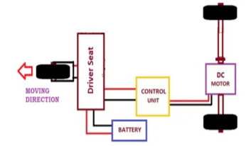
MATLAB MODEL :-

The model of the electric rickshaw is created in Simulink and is given below.

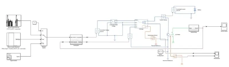
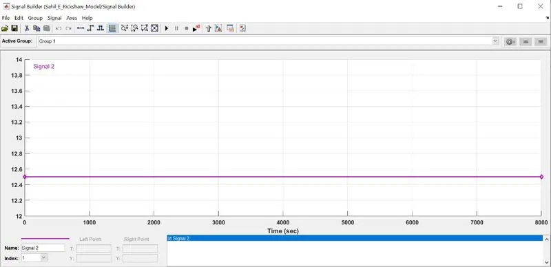
The model consists of three inputs which are 2 drive cycles the FTP75 and the Wide Open Throttle (WOT) cycles. The third input is a signal builder to satisfy the condition for the rise in temperature of the motor and controller at 45 Km/hr for 100 Km.

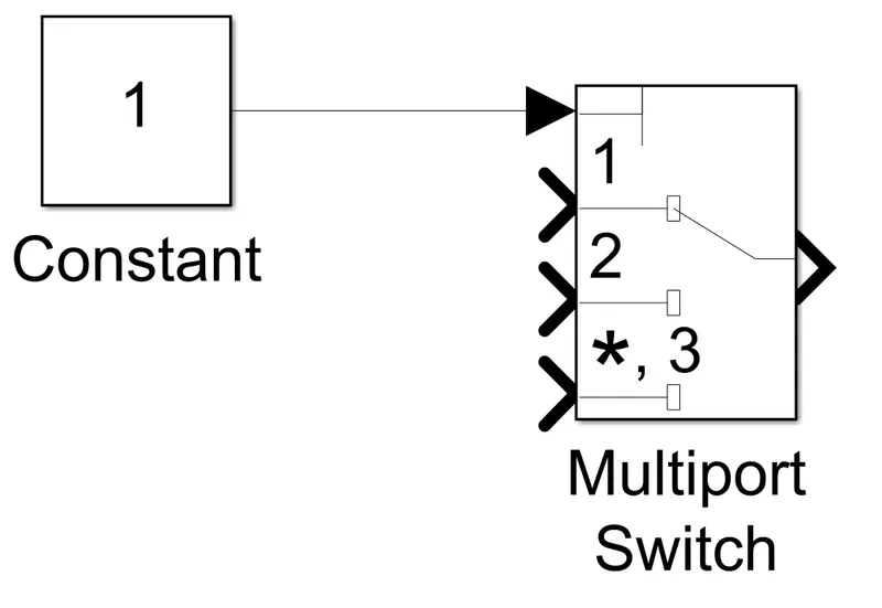
Either of the 3 inputs can be selected using the multiport switch. Here the number of input ports can be selected and a constant block is used to select the ports for the simulation.

The output port of the multiport switch is connected to the PID controller subsystem that controls the acceleration and braking of the vehicle. It is a simple alternative to the longitudinal driver block from the power train blockset.

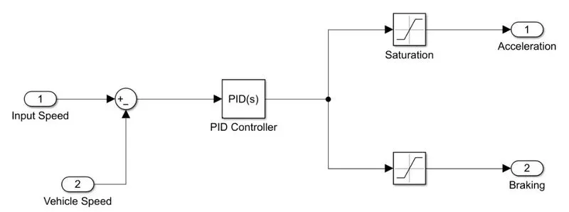
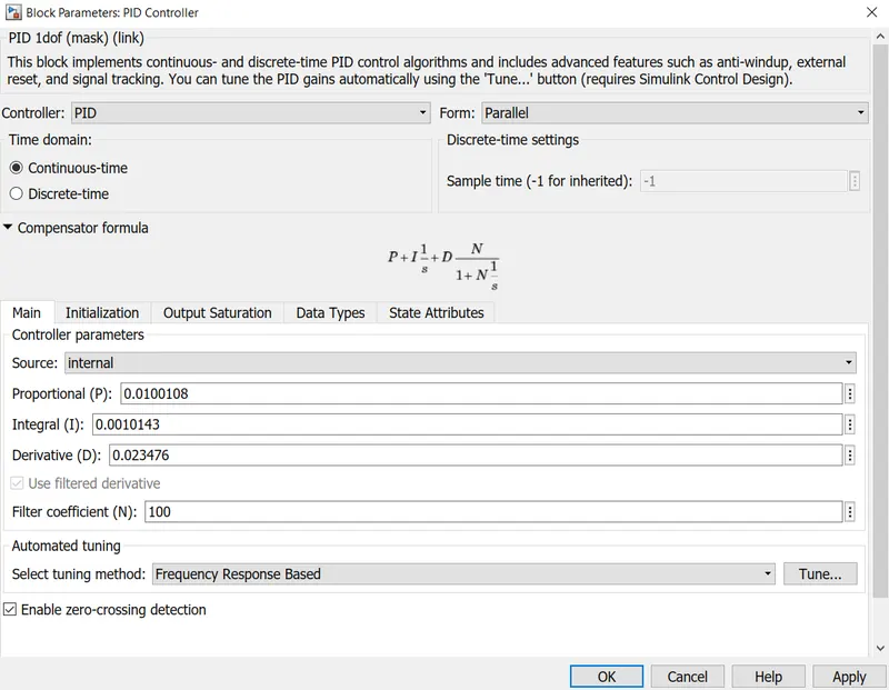
The input speed block is the port which is connected from the output of the multiport switch and the vehicle speed block is the input port which is connected from the output port of the vehicle body subsystem which is the feedback signal for the PID controller. The signal from the two inputs is passed through a sum block and it's output is then passed through the PID controller block where the gains of the P, I and D are entered. A saturation block each is used for the output of acceleration and braking to limit the input signal.

The output ports of the PID controller subsystem are connected to two controlled voltage source blocks.

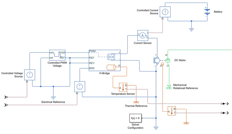
The output from the controlled voltage source which controls the acceleration signal is connected to a controlled PWM voltage block. This block creates a Pulse-Width Modulated (PWM) voltage across the PWM and REF ports. The output voltage is zero when the pulse is low, and is equal to the Output voltage amplitude parameter when high. Duty cycle is set by the input value.

The PWM and REF ports of the controlled PWM Voltage block is connected to the PWM and REF input ports of the H-Bridge block. This block is the controller for the DC motor. The block can be driven by the Controlled PWM Voltage block in PWM or Averaged mode. In PWM mode, the motor is powered if the PWM port voltage is above the enable threshold voltage. In Averaged mode, the PWM port voltage divided by the PWM signal amplitude parameter defines the ratio of the on-time to the PWM period. Using this ratio and assumptions about the load, the block applies an average voltage to the load that achieves the correct average load current. The Simulation mode parameter value must be the same for the Controlled PWM Voltage and H-Bridge blocks. For this simulation the averaged mode is selected for both the blocks.

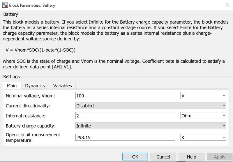
The second controlled voltage source block which controls the braking signal is connected to the BRK port of the H-Bridge block. The positive output port is connected to a current sensor block which converts current measured in any electrical branch into a physical signal proportional to the current. The physical signal of the current sensor block is connected to a controlled current source block which represents an ideal current source that is powerful enough to maintain the specified current through it regardless of the voltage across it. The controlled current source block is then connected to a battery block in a closed loop. The voltage of the battery block is set at 100 V and the same value is set for the controlled PWM voltage block, the H-Bridge block and the DC motor block. An electrical reference is added to ground the closed loop.

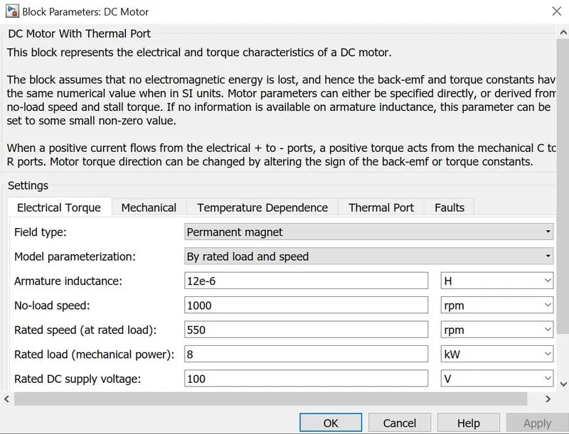
The electrical port of the current sensor is connected to the positive input port DC motor block. The DC motor block is configured to rated load and speed parameterization where the no load speed, rated speed, power and the output voltage are specified.

In order to plot the temperature rise of the motor and the controller a thermal port is required to be added to the blocks of the H-Bridge and the DC motor. Once the thermal ports are added they are connected to temperature sensor blocks which measures temperature in a thermal network. There is no heat flow through the sensor. The physical signal port T reports the temperature difference across the sensor. The measurement is positive when the temperature at port A is greater than the temperature at port B. The ports T are connected to thermal references and the ports B are connected to a scope to show the plot of the temperature rise.

A mechanical rotational reference is connected to the port C of the mechanical section of the DC motor block which is connected to ground the motor. The mechanical output port R is then connected to the gear port of the vehicle body subsystem.

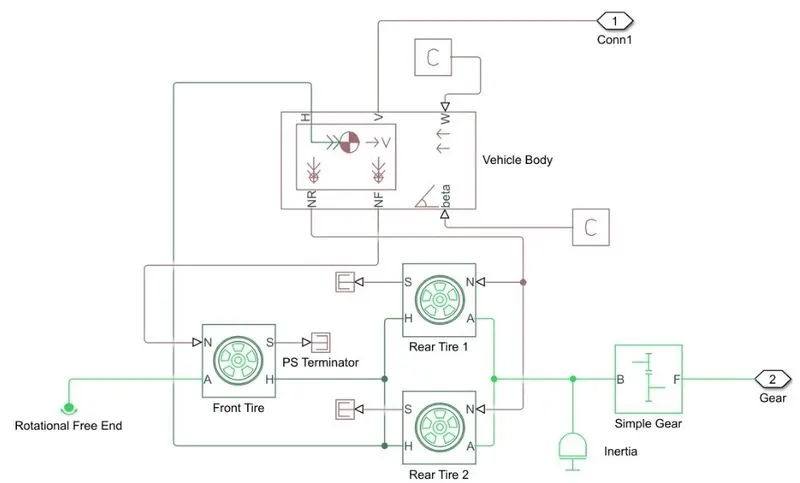
The subsystem consists a vehicle body block, 3 tire blocks and a simple gear block.

The vehicle body block represents a two-axle vehicle body in longitudinal motion. The block accounts for body mass, aerodynamic drag, road incline, and weight distribution between axles due to acceleration and road profile. The vehicle can have the same or a different number of wheels on each axle. Optionally include pitch and suspension dynamics or additional variable mass and inertia. The vehicle does not move vertically relative to the ground. Port H is a mechanical port which is connected to wheel hubs of the tire block and port V is the output port which shows the vehicle speed. Ports W and beta are for wind speed and surface inclination respectively and these two ports are connected to a PS Constant block with the value set to zero as they are not requried for the simulation.

The tire blocks used are the Magic Formula Tire blocks which represents the longitudinal behavior of a highway tire characterized by the tire Magic Formula. Connection A is the mechanical rotational conserving port for the wheel axle. Connection H is the mechanical translational conserving port for the wheel hub through which the thrust developed by the tire is applied to the vehicle. Connection N is a physical signal input port that applies the normal force acting on the tire. The force is considered positive if it acts downwards. Connection S is a physical signal output port that reports the tire slip.

Since a rickshaw is a rear wheel driven vehicle the rear tires are connected to the simple gear block which represents a fixed-ratio gear box. This simple gear block is the input block for the vehicle body subsystem where the output port R of the DC mtor is connected to the port F of the simple gear block and port B is connected to the rear wheels.

The port A of the front tire is connected to a rotational free end block as it is not driven by the motor and is used for steering. The ports N of the tire blocks are connected to the NF and NR ports which calculate the front and rear normal forces of the tires respectively. The vehicle body block then calculates the forces from the NR, NF and H ports and determines the vehicle speed through port V which is connected to the scope. The port V is also connected to the PID controller sub system to provide feedback to the PID controller.

The simulation is run for 3 different drive cycles and the following speed and temperature results are obtained.

1. FTP 75 drive cycle.

It is a drive cycle by the Environment Protection Agency (EPA) which is used measure tail pipe emissions and fuel economy of passenger vehicles.

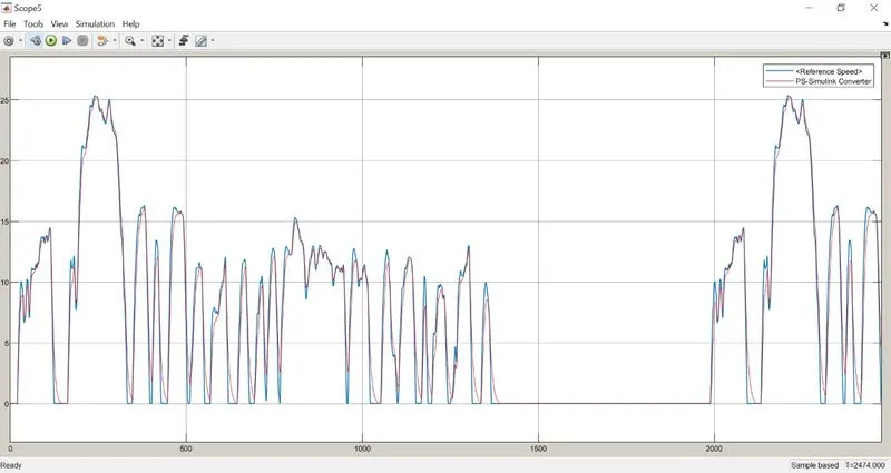
The output speed of the vehicle closely matches the input speed of the drive cycle, but there are variations in the output praticularly at the braking regions where the curve is smooth and gradual and not sharp.

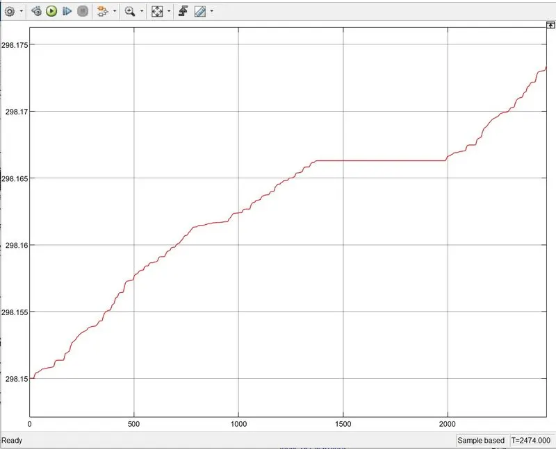
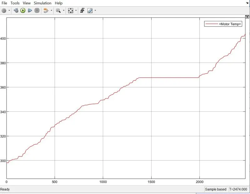
The two plots show the temperature of the controller and the motor. It can be observed that there is an erratic rise in the temperature when the battery is discharged during acceleration. During the coasting and braking period the battery temperature is stable at a constant rate and then starts to rise when the accelerator is pressed.

2. Wide Open Throttle (WOT) Drive Cycle.

In this drive cycle the throttle is opened at a 100% and full power and torque of the vehicle is utilised.

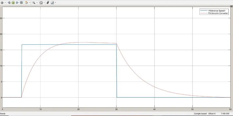
The variation in the vehicle speed to the input speed is observed because of the various parameters of the motor and controllers which affect the output.

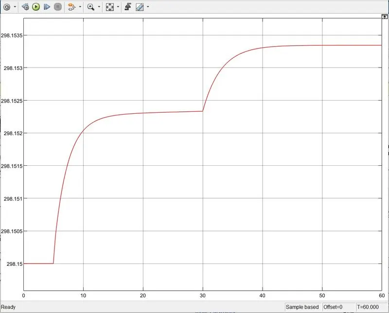
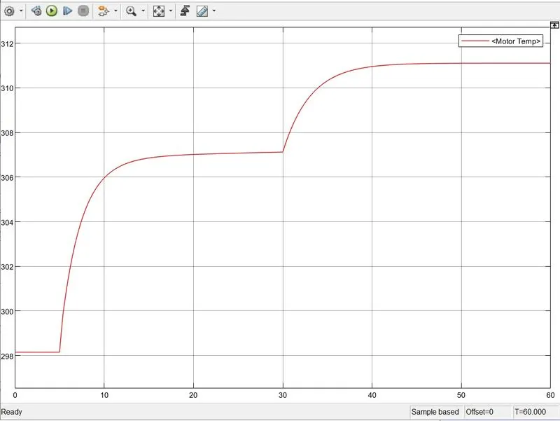
From the temperature plots it can be observed that the temperatures of the motor and the controller rise steadily in a parabolic nature during acceleration and stabilises to a constant temperature while braking.

3. Constant speed of 45 Km/hr for a distance of 100 Km travelled.

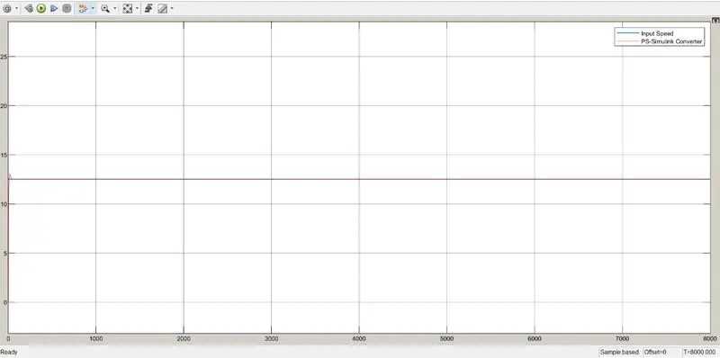
The output speed of the vehicle matches the input speed of the signal builder but there is a slight overshoot before the vehicle reaches the desired speed.

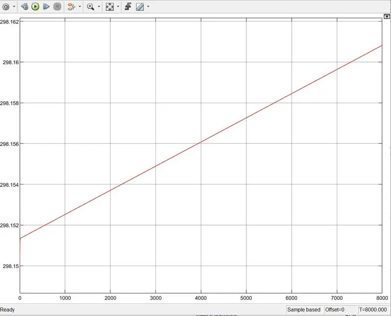
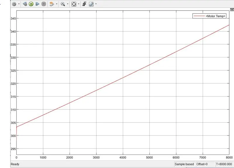
Since the rickshaw is travelling at a constant speed without braking or coasting the temperature of the motor and controller are increasing at a steady linear rate.

CONCLUSION :-

The Simulink model of an electric rickshaw is created and the vehicle speed and temperature rises of the motor and controller are plotted for three different drive cycles.