Week 4 Project - Simple Crank Mechanism

AIM :-

• To create and simulate a simple crank mechanism in Hyperworks.
• To determine the type of joint used for the slider section to prevent redundancy issues.
• To simulate the model with initial angular velocity and to plot the velocity vs time of the third joint with respect to the ground.
• To simulate the model by removing the angular velocity and applying a force on the second joint and to plot the reaction torque vs time.
• To add a bistop function for the first joint and simulate the model to plot the torque vs time.

GIVEN DATA :-

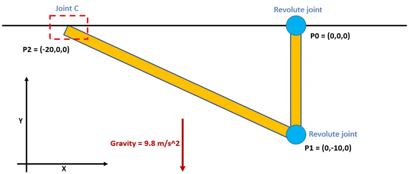
• Diameter of cylinders is 2 m.
• P0 and P1 have revolute joints.

CREATING THE MODEL :-

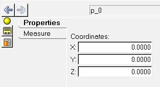
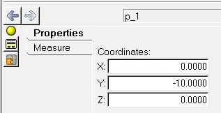
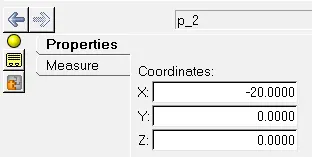
First three points are created, P0, P1 and P2.

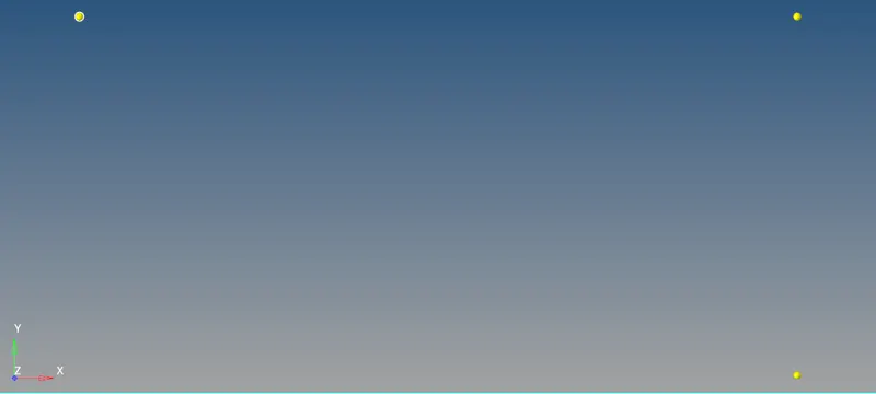
It is done by clicking on the add points option and the coordinates of the points are defined.

Two free bodies are created using the add bodies option. The properties of the free bodies are defined later after the cylinders are created.

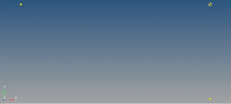
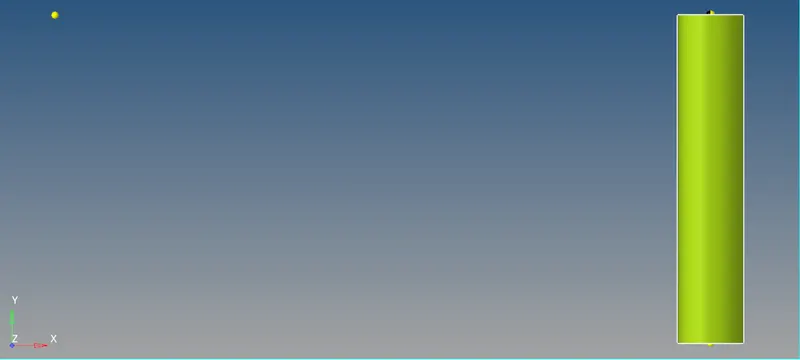
To create the cylinders, the add graphics option is selected.

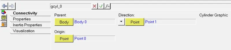
The first cylinder is created by defining the parent, origin and direction under connectivity as shown below.

The second cylinder is created by selecting another graphic and defined by selecting the parent origin and direction under connectivity.

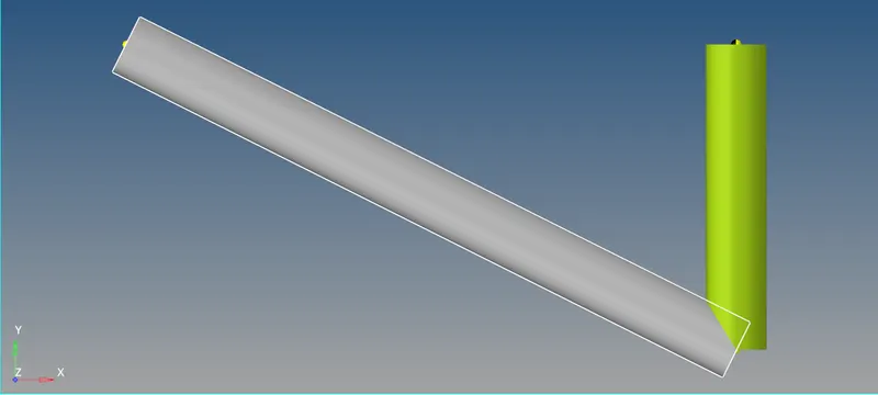
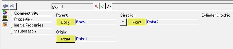
For both the cylinders, the diameter is 2 m. This is defined by specifying the radius as 1 m.

In order to shift the free bodies to center of mass and to obtain it's properties, the get properties from associated graphic(s) is selected.

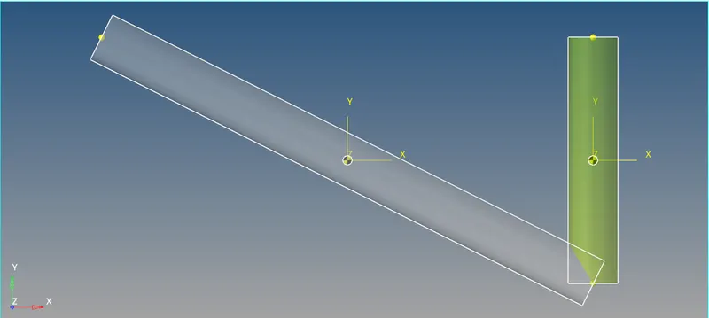
This shifts the free bodies to the center of mass and the mass and inertial values are defined.

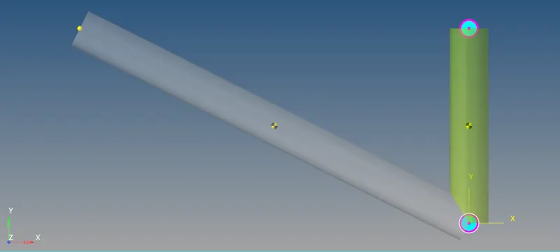
The revolute joints are created at P0 and P1. This is done by selecting the add joint option.

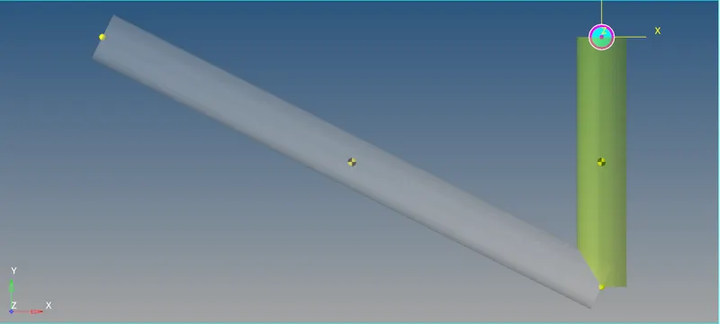
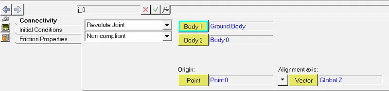
The joint at P0 is created by defining the bodies, origin and alignment axis under connectivity.

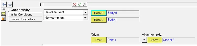
Another revolute joint is created at P1 and the bodies, origin and alignment axis under connectivity is defined.

1. WHAT TYPE OF JOINT MUST BE GIVEN AT P2 SO THAT THE SYSTEM DOES NOT HAVE REDUNDANCY ISSUES? :-

The joint at P2 will act as the slider. The system has 2 rigid bodies with each having 6 degrees of freedom which would result in a total of 12 degrees of freedom. The revolute joint has 5 degrees of freedom which would result in a total of 10 degrees of freedom. If a translational joint is used, it would make the system redundant as it has 5 degrees of freedom which would result in a total of 15 degrees of freedom removed when the 2 revolute joints are added. This would end up with a total degree of freedom of -3 which makes the system over constrained as shown below.

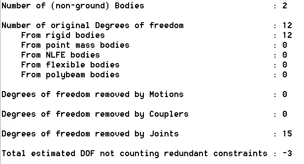
In order to remove the redundancy issue, an inline joint is used. The inline joint has 2 degrees of freedom which when added with the revolute joints will result in the degrees of freedom removed by the joints to be 12. Therefore the total degrees of freedom would be 0 which removes the redundancies and makes the system completely constrained as shown below.

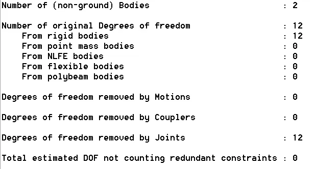
Therefore, the inline joint is the right joint to be used for P2.

2. AFTER SELECTING JOINT C, SIMULATE THE MECHANISM WITH AN INITIAL ANGULAR VELOCTY OF 0.5 rad/s AT P0 AND PLOT THE GRAPH FOR VELOCITY VS TIME FOR P2 WITH RESPECT TO THE GROUND. FIND THE MAXIMUM VELOCITY AND WHAT IS THE CHANGE IN THE DEGREES OF FREEDOM :-

The angular velocity is provided by going to initial conditions of joint 0 and then by selecting rotation. The value of 0.5 rad/s is provided under velocity as shown below.

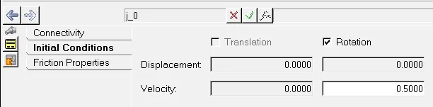
An output is created to plot the graph using the add output option. Under properties velocity is selected and the bodies, reference marker and the points are defined as shown below.

The model is saved and the simulation is run for 20s. After the simulation is completed, the graph of the velocity vs time at P2 with respect to the ground is plotted.

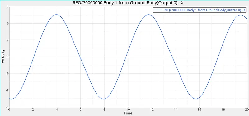
The maximum velocity can be obtained by selecting the statistics option. This provides details about the plot as shown below.

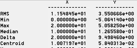
The maximum velocity of P2 is 5.058 m/s.

The degree of freedom remains the same.

3. SUPRESS THE INITIAL ANGULAR VELOCITY AND APPLY A LOAD OF 1000 KN AT P1. PLOT A GRAPH OF THE REACTION TORQUE VS TIME AT P0 :-

The angular velocity is removed by deselecting the rotation option under initial conditions. A force is created using the add force option on the client specific toolbar.

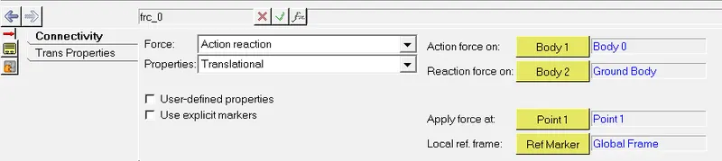
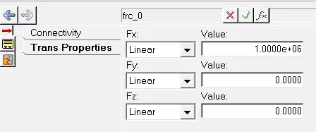
The force is selected to action-reaction and translational force is selected under properties. The body and point upon which the force acts on is defined. To define the load value, the force acting on the x-direction is selected and since the load is 1000 KN, 1e+6 is entered in the value dialouge box.

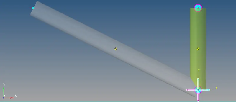
The force is represented in the model as shown below.

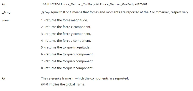
In order to obtain the reaction torque, an output is created and expressions is selected. Then the expression builder is selected and a VTORQ expression is created. The VTORQ function returns the specified component of the force or torque applied by the force vector. The format for VTORQ expression is,

VTORQ(ID, JFLAG, COMP, RM) where,

The expression to calculate the reaction torque is given below,

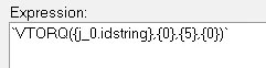
Where,

ID = j_0.idstring which is the ID string of joint 0 or P0.

JFLAG = 0 which is the force at the i marker.

COMP = 5 which is the torque magnitude.

RM = 0 which is the global frame.

Once the expression function is created as an output, the simulation is run and the graph of the reaction torque vs time of P0 is plotted as shown below.

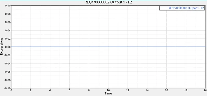
The plot shows that there is no reaction at P0 during the entire simulation.

4. WITH THE SAME APPLIED FORCE AT P1, CREATE A BISTOP FUNCTION AT P0 WITH THE RANGE OF -10 TO 0 DEGREES AND PLOT THE GRAPH OF THE REACTION TORQUE VS TIME AT P0 :-

A second force is created where the type of force is action-reaction but here rotational force is selected. The body and point upon which the force acts on is defined which in this case is P0.

The BISTOP function is defined under rotational properties which is done by selecting expression from the drop down options under Tx which is rotation in the x-direction and the function builder is opened.

A BISTOP function is one that models a gap element. It can be used to model forces acting on a body while moving in the gap between two boundary surfaces, which act as elastic bumpers. The properties of the two boundary surfaces can be tuned as desired. The format for a BISTOP function is,

Bistop(x,˙x,x1,x2,k,e,cmax,d) where,

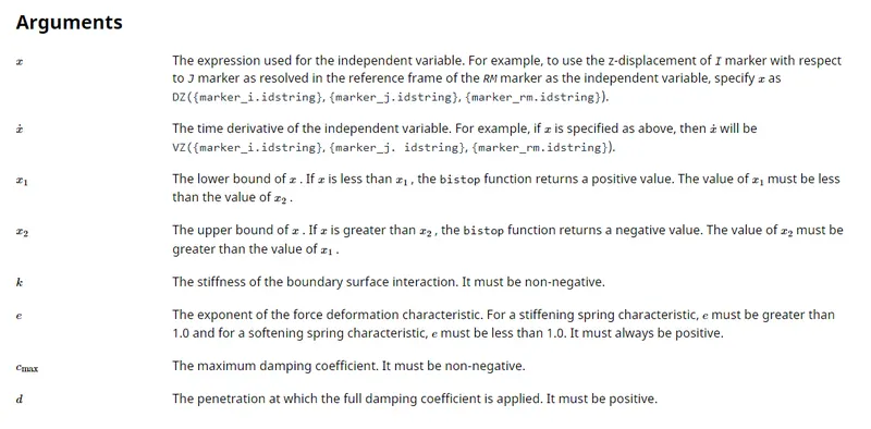
The BISTOP expression created as the rotational input at P0 is given below.

The ID strings for the I and J markers of J0 is defined in the AZ and WZ direction which are the translational and rotational directions respectively. The angle range is defined and converted to radians. The stiffness, damping and penetration are also defined.

A new output is created as a VTORQ expression to plot the reaction torque.

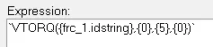
Here instead of J0 the force with the BISTOP function is defined as the ID.

The simulation is run and the graph of the reaction torque vs time at P0 is plotted.

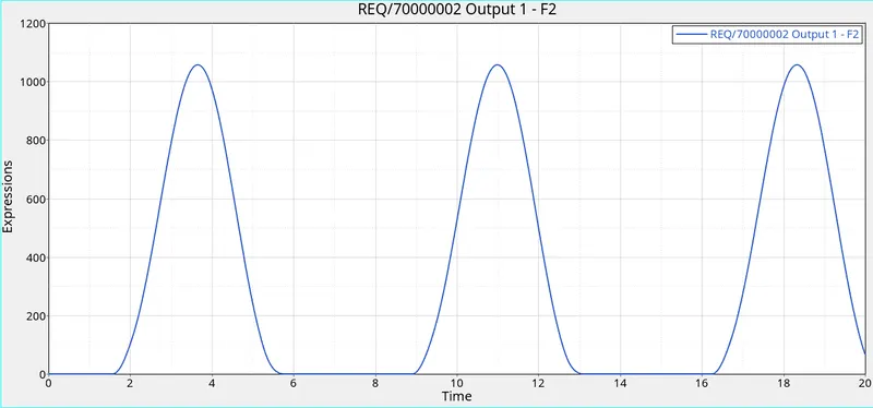
The graph shows the variation in the reaction torque as P0 moves from -10 to 0 radians.

CONCLUSION :-

• A model of a simple crank mechanism is created in hyperworks.
• A joint at P2 or the slider is detemined to avoid redundancy issues.
• An angular velocity is provided and the velocity vs time of P2 is plotted.
• After the angular velocity is suppressed, a force is created and the reaction torque vs time of P0 is plotted with the help of a function expression.
• While retaining the same force, a new force is created using the BISTOP function and the reaction torque vs time of P0 is plotted.