Project

AIM :-

The aim of this project is to analyse the simulink model of an all terrain vehicle.

OBJECTIVES :-

The models which will be studied are,

• Model of the ATV.
• Model of the ATV with a dashboard to vary the input parameters.
• Model of the ATV with a go-to block to store the gear ratios.
• Model of the ATV with a look-up table.
• Model of the ATV with a look-up table and a dashboard.

THEORY :-

An all-terrain vehicle (ATV) is defined as a motorized off-highway vehicle designed to travel on four low-pressure or non-pneumatic tires, having a seat designed to be straddled by the operator and handlebars for steering control. THese vehicles are used to travel of rough terrain for recreational or racing purposes.

The major difference between a BAJA ATV and a conventional ATV or a quad bike is that the BAJA is built as a buggy. The chassis consists of a roll cage, with pedal mounted controls for acceleration and braking and a steering wheel to turn the vehicle as opposed to a handle bar used in a quad bike.

The transmission used to transmit the power to the driven wheels is a Continously Varying Transmission (CVT). This type of an automatic transmission is pulley driven compared to the conventional gear driven automatic transmission.

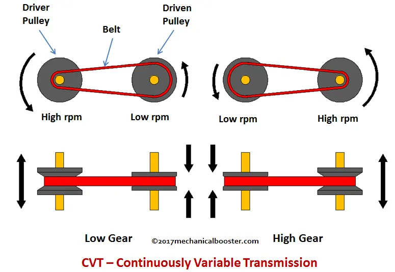
A CVT gearbox has a relatively simple arrangement of two cone-shaped pulleys with a V-shaped drive belt connecting them. One pulley is attached to the engine, while the other is joined to the wheels. When you press the accelerator, the engine revs and the cone moves according to the amount of power asked for. The other cone adjusts accordingly so that the drive belt maintains the same tension, and this is what determines how the car accelerates. As the two cones move independently, that means there are no set gear ratios as you would find in a conventional auto or manual, so a CVT is, in effect, a single-speed unit with infinite gear ratios available.

A CVT gearbox doesn't have many moving parts, so it's relatively reliable. It's also mainly used in low-power applications, so cars running a CVT are usually fairly unstressed.

SIMULINK MODEL :-

1. ATV Model.

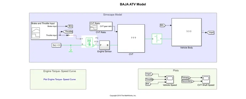
Above is a model of the ATV with a CVT. The model consists of two subsystems which contain the simulink models of the CVT and the vehicle body.

Explanation of the model,

A signal builder is used to create input signals for the throttle, brake and the gear ratio of the CVT.

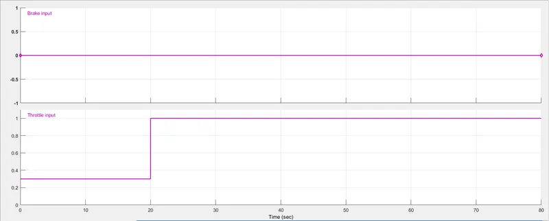
Here the input provided for the brakes is set constant at 0. For the throttle input it starts at 0.3 for 20s and then increases to 1 for the remainder of the time.

These input signals are then connected to a generic engine block.

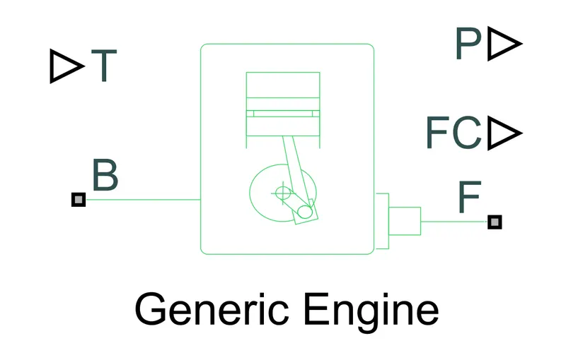
This block represents a system level model of a spark ignition or compression ignition engine. The throttle input signal T lies between 0 and 1 which specifies the torque demanded from the engine as a fraction of the maximum possible torque. Connection port B is the mechanical rotational conservation port which represents the engine block. The solver configuration block and the rotational reference blocks are connected to this port. The connection port F is the mechanical rotational conservation port which represents the engine crankshaft. Connections P and FC are the physical signal output ports which represent power and fuel consumption respectively.

The port P is connected to a sub-system called engine sensor which is used to obtain the engine's rpm.

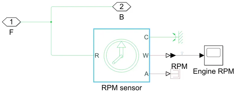
Here the rpm sensor is an ideal rotational motion sensor block. with the inputs being ports F and B which is connected to port R. The rotational reference is connected to the port C which is the negative reference port of the motion sensor. The engine's rpm is provided through the port W which is a pysical signal port that represents angular velocity.

The next subsystem that is created is the CVT system. For the input signal a signal builder is used to build the input of the gear ratios.

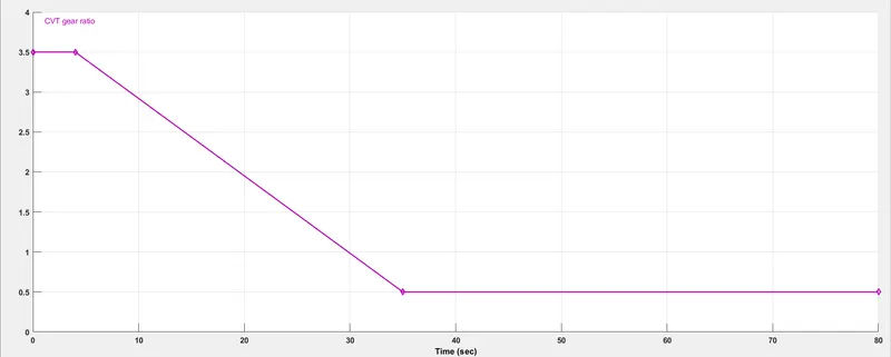
The initial gear ratio is 3.5 for about 5s and then linearly decreases to 0.5 between 5s to 35s. It maintains a constant ratio of 0.5 from 35s onwards. Here 3.5 is the gear ratio required to move the vehicle. As the speed increases the gear ratio decreases and reaches overdrive at 0.5.

The CVT subsystem is given below,

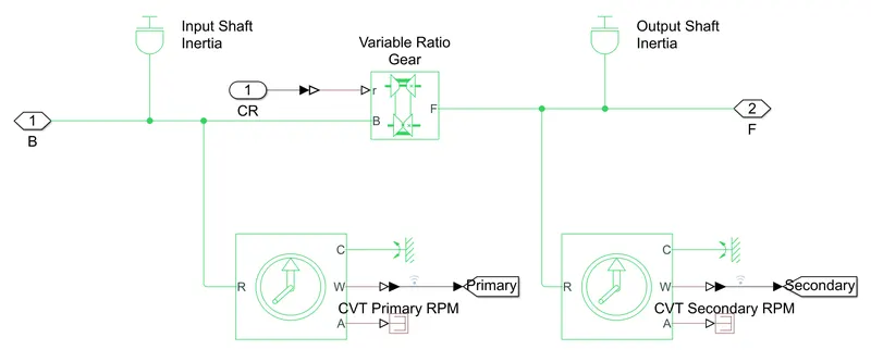
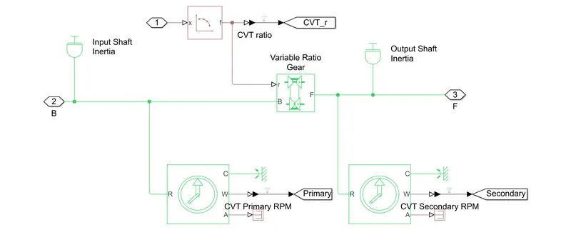
This model has two inertia blocks for the input and the output. These two blocks represent the ideal mechanical rotational inertia of the system. The main block of this system is the variable ratio transmission block which represents the CVT.

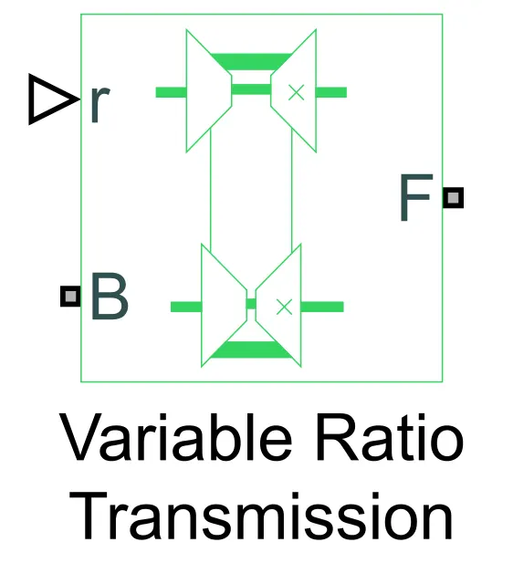
The port r is the physical signal input which defines the ratio of input to output angular shaft velocities. Port B is a rotational conserving port which stands for base and connects the primary (driving) cone of the transmission and port F is a rotational conserving port which stand for follower and connects the secondary (driven) cone of the transmission. Two ideal rotational motion sensors are used to calculate the rpm of the the primary and secondary cones when the gear ratios change.

A simple gear block is used to connect the CVT and vehicle body sub system. The subsystem of the vehicle body is given below.

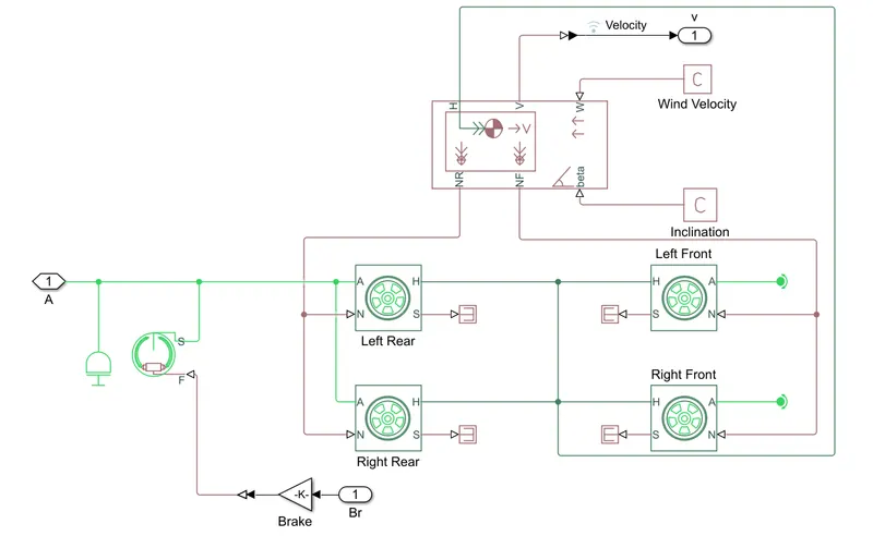
The blocks used in the subsystem are vehicle body, double shoe brake and tire blocks.

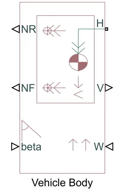
This block represents a two axle vehicle body in longitudinal motion. This block accounts for body mass, aerodynamic drag, road incline and weight distribution among the axles. Connection H is the mechanical translational conserving port which represents the horizontal motion of the body. The net traction developed by the tires is connected to port H. Connections NF and NR are the physical signal output ports for the normal front and normal rear wheel forces respectively. Connection V is the physical signal output port which provides the velocity of the vehicle. Connection W is a physical signal port that represents the wind speed and connection beta is a physical signal port that represents the inclination of the road. The vehicle body block also allow for the conditions of vehicle drag to be added as a parameter.

The tire block is used to represent the tires of the ATV. They are connected to the NF and NR ports of the vehicle body block.

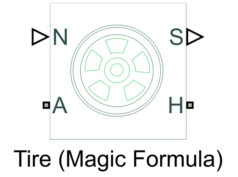
This represents the longitudinal behaviour of a tire. Connection A is the mechanical conserving port for the wheel axle, the input signal is connected to this port. Connection H is the mechanical conserving port for the wheel hub through which the thrust developed by the tire is applied to the vehicle. This port is interconnected with the other tire blocks. Connection N is the physical signal input which applies the normal force acting on the tire. Here force is positive if it acts downwards. Connection S is a physical signal output port that represents tire slip. In this model we use a Physical Signal Terminator block as we do not need to find the tire slip.

Brake block is used to represent the braking force acting on the vehicle.

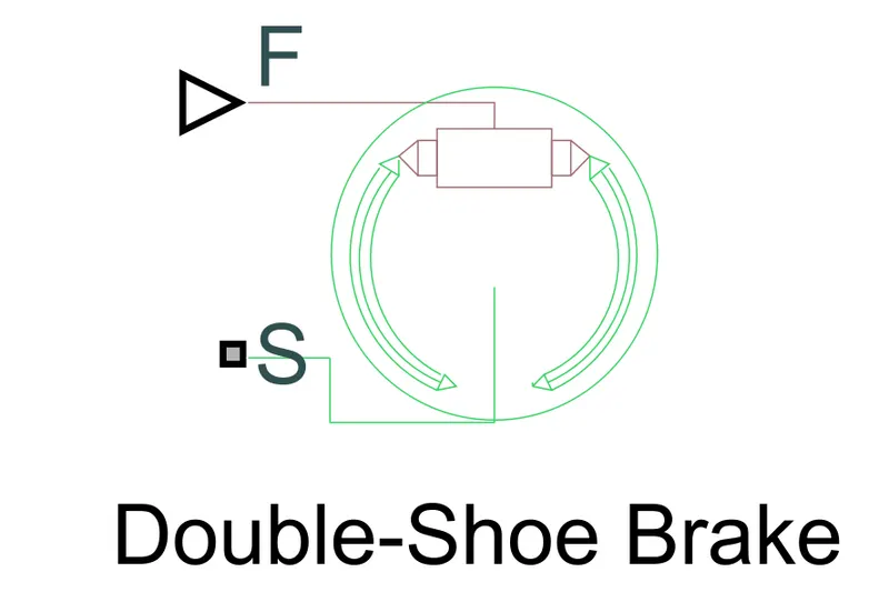
Here connection F is the physical signal input which is used to activate the actuator. Connection S is a rotational terminal port which represents the drum shaft. This port is connected to the port A of the tire block.

The combination of the signal builders, engine block, CVT subsystem, simple gear block, and the Vehicle Body subsystem comprise of the ATV model.

2. ATV Model with a Dashboard.

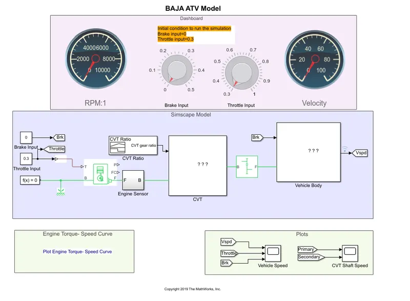
The major difference in this model is that there is no signal builder for the throttle and brake inputs. Instead circular gauges are used to represent the engine speed and vehicle speed and knobs are used to vary the throttle and brakes. Constant blocks are used to link the throttle and brake knobs to the simulink model.

3. ATV model with a go-to file.

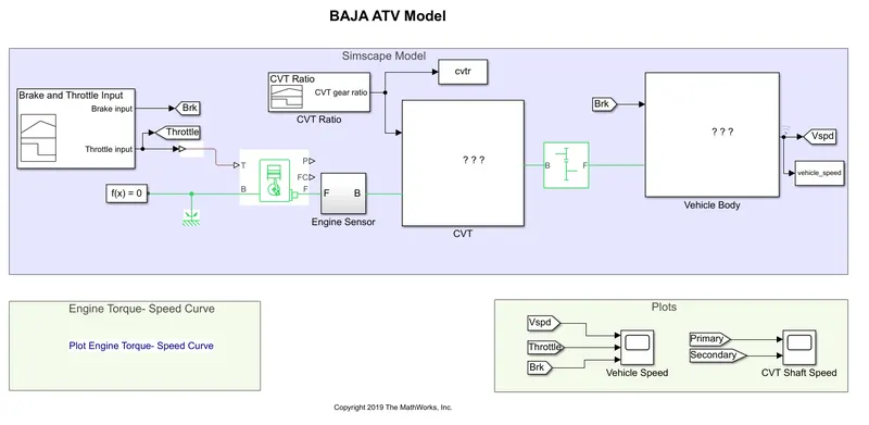
The model has a go-to block for storing the input values of the gear ratios for the cvt transmission in the MATLAB workspace. Once the simulation runs the results get stored in the workspace in a table. This data stored in the workspace is then used as the input for the look-up table.

4. ATV Model with a Look-up Table.

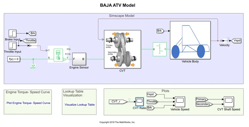
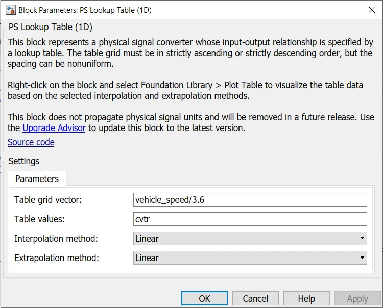
Here the signal builder inputs are removed. For the throttle and transmission the step blocks are used as inputs where the initial and final values are defined with the exception of the brake input signal where the values are a constant zero. Here the values periodically increase over time when the simulation is run. The input signal of the CVT transmission is provided in the form of a look-up table.

The table values are defined as cvtr which are the gear ratios stored in the MATLAB workspace.

5. ATV Model with a Look-up Table and Dashboard.

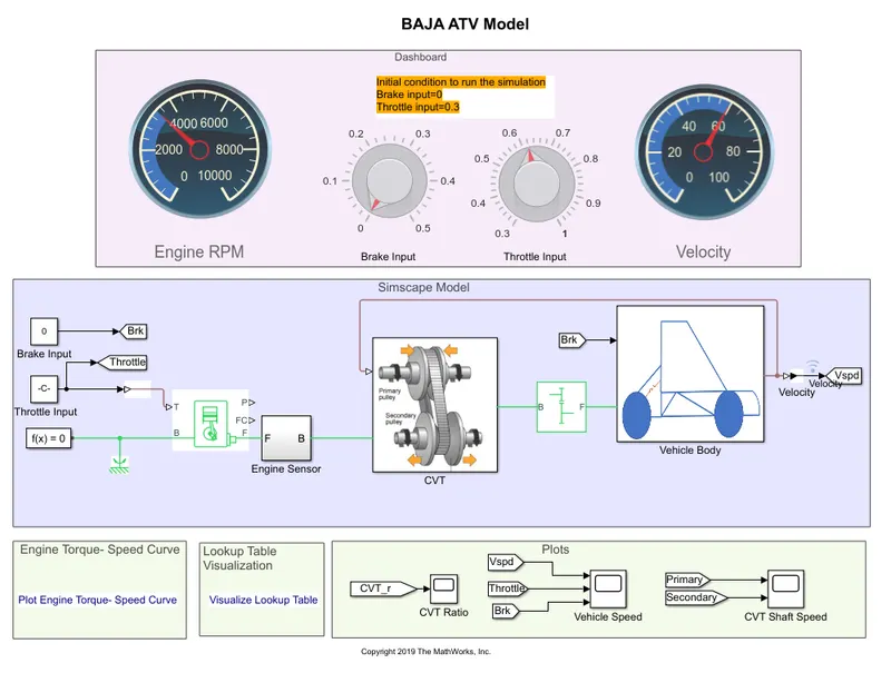
Here the step blocks are removed for the input of the throttle and brake, and constant blocks are added. These constant blocks are linked to the knob blocks for the user to manually vary the throttle and brake inputs while the simulation is running.

RESULTS :-

1. ATV Model.

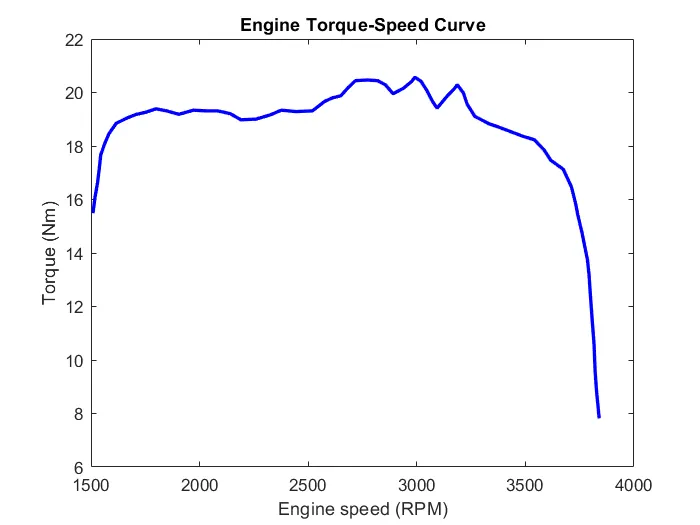
The torque-speed curve of the engine is used to determine the input parameters of the vehicle. From the graph we can see that the vehicle reaches a peak torque of 20 Nm at 3000 rpm and starts to fall and reaches a maximum rev limit of 3850 rpm.

The next plot is that of the vehicle speed when acceleration is provided.

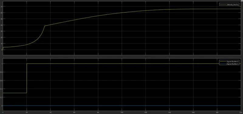
The first graph represents the speed of the vehicle and the second graph represents the throttle and braking inputs. Here the brake input is constant. For 20s we have a constant throttle input of 0.3 where the speed of the vehicle gradually increases to about 8 Km/hr. Once a full throttle is provided the speed drastically increases till it attains a max speed of 60 Km/hr.

The second plot is of the speed of the CVT cones.

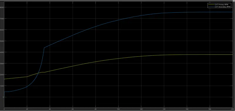
Here the yellow line represents the speed of the primary of driving pulley and the blue represents the speed of the secondary or driven pulley of the transmission. When the vehicle starts to move the primary pulley's speed is higher than the secondary pulley's speed. As the speed of the vehicle increases, the belt moves over the pulleys and the speed of the secondary pulley increases significantly over the primary pulley.

2. ATV model with a dashboard.

By being able to vary the throttle input using the knob block, the following graphs were obtained.

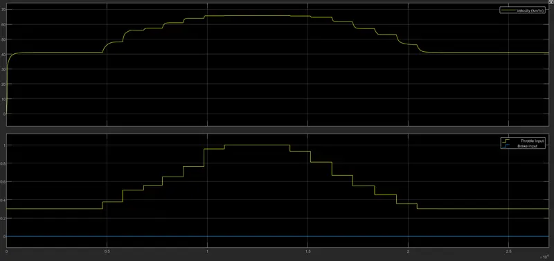
The upper graph is the speed of the vehicle. The lower graph has the throttle and brake inputs. Here the brake input is at a constant 0. It can be observed that the speed increases proportionately as the throttle is increase to 1 and brought back to the initial condition of 0.3.

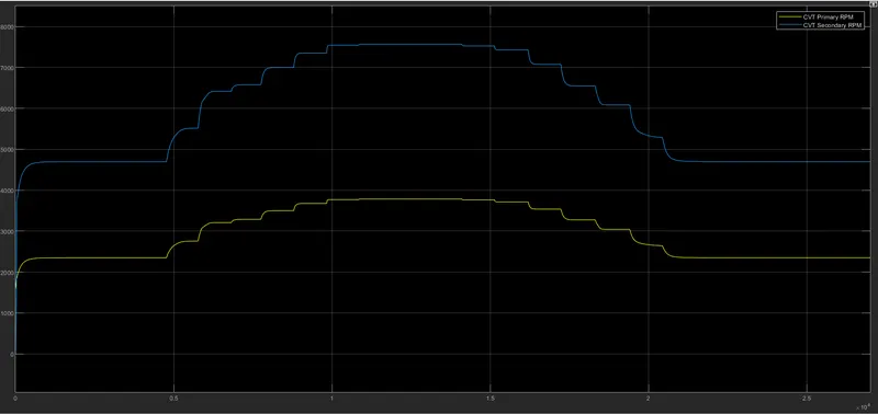
In the above graph we can see the change in the pulley speeds of the CVT transmission as the throttle is varied from initial condition to final condition and back. It can be observed that as the vehicle reaches top speed, the secondary pulley's speed increases greatly compared to the primary pulley.

3. ATV model with a go-to file.

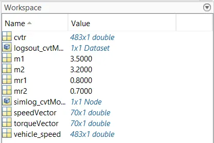
The gear ratios are stored in a table called cvtr in the workspace as a table.

4. ATV Model with a Look-up Table.

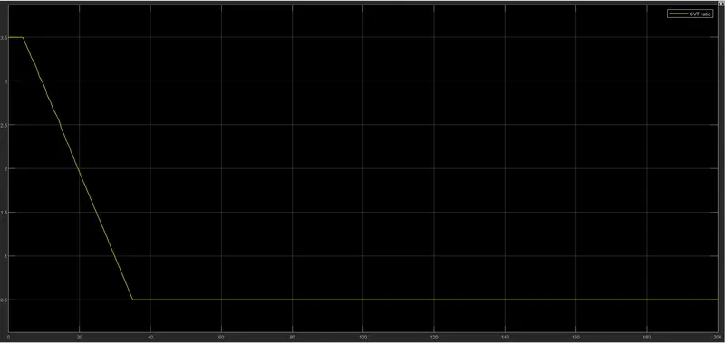
The above plot is the gear ratio of the CVT from the lookup table, where it starts at 3.5 and decreases to 0.5 when the vehicle is in overdrive.

The graph of the vehicle speed and the CVT pulleys speeds remain the same as of the first case where a signal builder is used for input.

5. ATV Model with a Look-up Table and Dashboard.

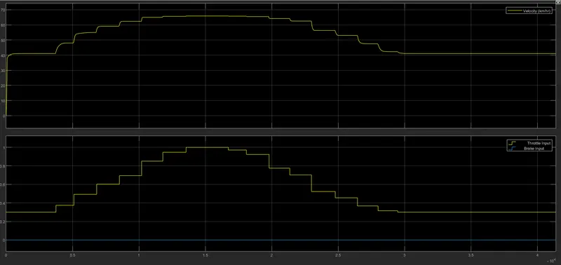
The above plot shows the change in speed when the throttle input is varied from initial value to final value and back.

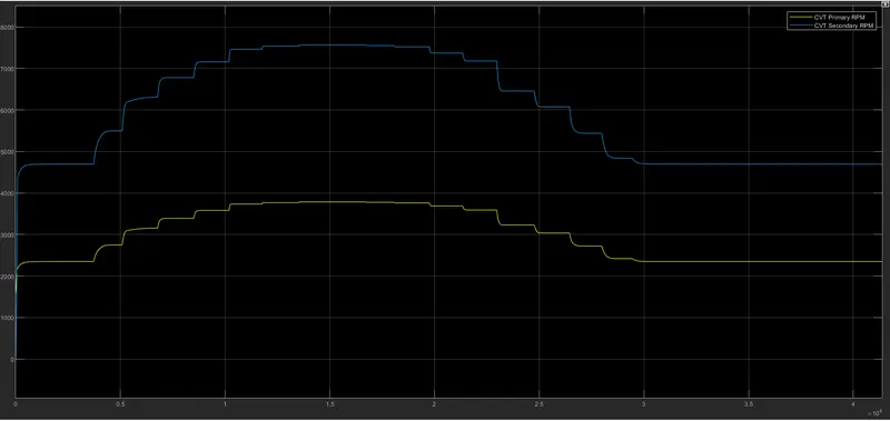
The variation of the CVT pulleys is observed as the throttle is varied.

CONCLUSION :-

The simulink model of the All Terrain Vehicle has been studied and it's graphs have been plotted.