Week 3 - Solving second order ODEs

Aim :-

To solve a 2nd Order Differential Equation of a simple pendulum using MATLAB.

Objective :-

• To write a program to solve the ODE of the motion of a simple pendulum using MATLAB.
• Plot the graph of the displacement and velocity.
• Create a simulation of the pendulum in motion.

Theory :-

A 2nd Order Differential Equation is an equation involving the unknown function y, its derivatives y' and y'', and the variable x. Which is written as,

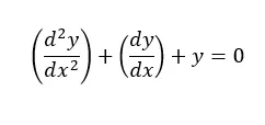
This linear equation helps us in understanding different engineering phenomenon and principles. Here we shall consider the motion of a simple pendulum through a 2nd Order Differential Equation.

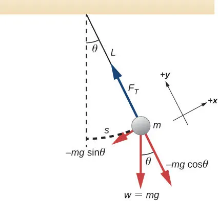
A simple pendulum consists of a bob of mass m suspended by string with negligible mass of length l. The forces that act on the pendulum are gravitation force g and the tension of the string.

Formulae :-

The 2nd Order Differential equation is defined as,

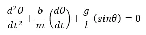
Where,

b = damping coefficient.

m = mass of the bob in Kg.

g = the gravity in m/s^2.

l = length of the string in m.

Breaking down the 2nd Order Differential Equations into two 1st Order Differential Equations,

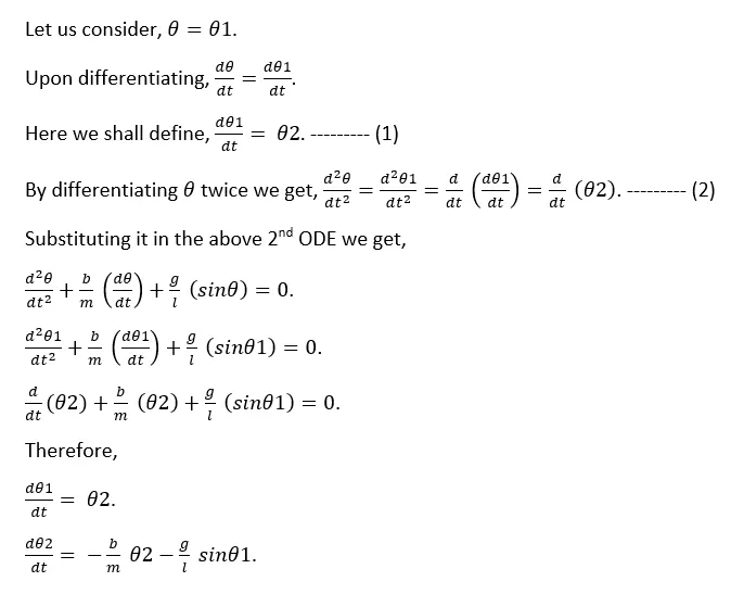
From this derivation we have defined θ1 and θ2.

Program :-

First a function to define the 2nd Order Differential Equation for defining θ1 and θ2 is written.

% ODE function 
function [dtheta_dt] = ode_func(t,theta,b,g,l,m)

        theta1 = theta(1)
        theta2 = theta(2)
        dtheta1_dt = theta2;
        dtheta2_dt = -(b/m)*theta2 - (g/l)*sin(theta1);
        dtheta_dt = [dtheta1_dt ; dtheta2_dt];
end

After this, the main program to solve the 2nd Order Differential Equation is written.

%Solving second order differential
close all
clc

%Inputs
b = 0.05;
g = 9.81;
l = 1;
m = 1;

%Initial condition
theta_0 = [0;3];

%Time points
t_span = linspace (0,20,500);

%solve ODE
[t, results] = ode45(@(t,theta) ode_func(t,theta,b,g,l,m),t_span,theta_0);

%Plotting the graph
plot(t,results(:,1))
hold on
plot(t,results(:,2))
xlabel('Time')
ylabel('Plot')
legend("Angular displacement","Angular velocity")

% Writing a for loop to make the animation
ct = 1;
for i = 1:length(results(:,1))
    x0 = 0;
    y0 = 0;
    
    x1 = l*sin(results(i,1));
    y1 = -l*cos(results(i,1));
    % Plotting the animation
    figure(2)
    plot([-1 1],[0 0],'linewidth',5)
    hold on
    plot([x0 x1],[y0 y1],'linewidth',3)
    hold on
    plot(x1,y1,'o','markersize',20,'markerfacecolor','y')
    axis([-2 2 -2 2])
    pause(0.03)
    hold off
    M(ct) = getframe(gcf);
    ct = ct+1;
end

% Converting the animation into a movie
movie(M)
videofile = VideoWriter('pendulum_oscillation.avi','Uncompressed AVI');
open(videofile)
writeVideo(videofile,M)
close(videofile)

Explanation :-

For the first program, the function is defined based on the derivation to split the 2nd Order Differential Equation into two 1st Order Differential Equation. Once θ1 and θ2 are defined, they are stored as a solution vector where, dtheta_dt = [dtheta1_dt ; dtheta2_dt]; is a column matrix.

In the main program, the initials conditions of angular displacement and velocity must be provided to solve the ODE.

Here, theta_0 = [0;3]; defines the initial conditions with the displacement being 0 and the velocity being 3.

The ODE is integrated in order to obtain the solution. The time span is defined using a linear spaced array, t_span = linspace (0,20,500); where the time is taken between 0 to 20 seconds.

ode45 is an inbuilt solver in MATLAB used to integrate differential equations. To solve the differential equation we use an anonymous function.

Anonymous functions are those functions which are not stored as a function file, but it is a data type which uses the 'function handle' data type. Anonymous functions are declared directly in the main program.

[t, results] is the function handle of the anonymous function. @(t,theta) is the input argument of the anonymous function and ode_func(t,theta,b,g,l,m),t_span,theta_0 is the definition of the anonymous function. Using the ode45 command, the function is solved.

The graph is then plotted from the solution obtained.

To create the animation of the pendulum a for loop is written where the initial and final positions are defined. The animation is then plotted and converted to a movie using the videoWriter command.

Result :-

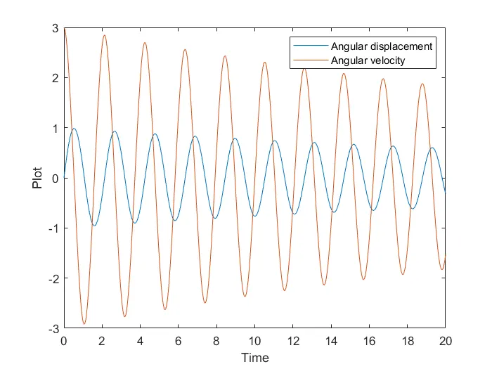
The graph of the angular displacement and velocity over time has been obtained. Due to a low damping coefficient it can be observed that the oscillations are strong.

https://drive.google.com/file/d/1MkuDiZ1ahAZKDeO6L_AGDV10FBnF3oiW/view?usp=sharing

The above link contains the video of the pendulum in motion.

Conclusion :-

We were able to solve the 2nd Order Differential equation of a pendulum in motion using MATLAB.

From the solution we were able to plot a graph of the oscillation of the pendulum.

We were also able to create a video of the pendulum in motion.