Vehicle Ride 1
AIM :-
- To calculate the frequencies for front and rear springs based on the three load conditions from the given parameters.
- To plot the bump oscillation profile for all three load conditions using MATLAB.
1. CALCULATE THE FREQUENCIES FOR FRONT AND REAR SPRINGS BASED ON CURB WEIGHT, HALF LOAD AND GROSS VEHICLE WEIGHT CONDITIONS :-
The parameters to be taken into consideration are given below.
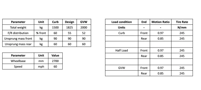
Also,
Front sprung mass natural frequency at half load, Ff = 1.15 Hz. This frequency is used for curb weight and gross vehicle weight loads.
Calculations,
a). Recommended rear sprung mass frequency based on speed and wheelbase at half load condition,
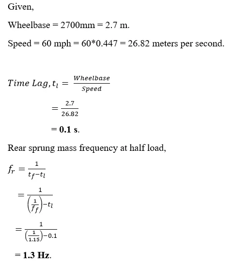
b). Front sprung mass natural frequency at half load,
The front sprung mass natural frequency at half load is Ff = 1.15 Hz.
c). Front spring rate,
The formula to calculate the spring rate is given as,
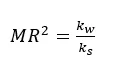
Where,
MR = Motion ratio.
Kw = Wheel rate.
Ks = Spring rate.
The wheel rate is an unknown variable and it obtained from the relation between the ride rate and tire rate which is given as,
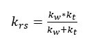
Where,
Krs = Ride rate of the sprung mass.
Kt = Tire rate.
The ride rate at sprung mass is calculated as follows,
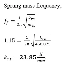
The wheel rate is calculated as follows,
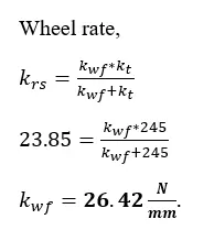
Once the wheel rate is obtained the spring rate is then calculated using the motion ratio formula,
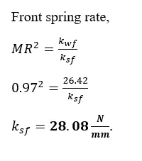
d). Rear spring rate,
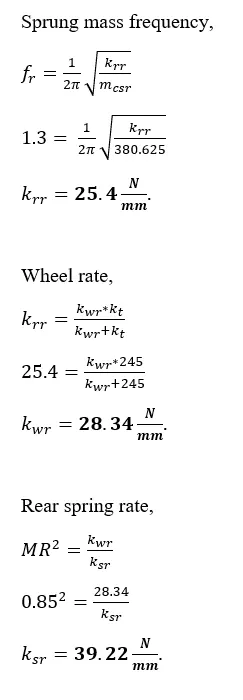
e). Front sprung mass natural frequencies at curb and GVW,
Sprung mass frequency is given as,
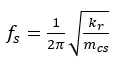
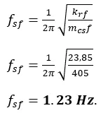
At curb weight we know that,
Krf = 23.85 N/mm.
mcsf = 405 Kg.
Therefore,
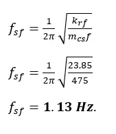
At GVW we know that,
Mcsf = 475 Kg.
Therefore,
f). Rear sprung mass natural frequencies at curb and GVW,
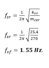
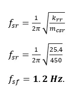
We know that, Krr = 25.4 N/mm.
For curb weight,
Mcsr = 270 Kg
For GVW,
Mcsr = 450 Kg.
g). Front unsprung mass natural frequency at all 3 load conditions,
The formula to calculate the unsprung mass frequency at all 3 load conditions is given as,
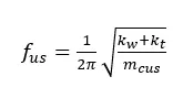
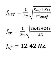
We know that,
Wheel rate, Kwf = 26.42 N/mm and ktf = 245 N/mm.
Corner unsprung mass, Mcusf = 45 Kg.
h). Rear unpsrung mass natural frequency at all 3 load conditions,
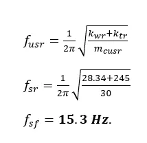
We know that,
Wheel rate, Kwr = 28.34 N/mm and tire rate, Ktr = 245.
Corner unsprung mass, Mcusr = 30 Kg.
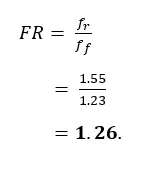
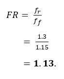
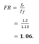
i). Rear/front frequency ratio for all 3 load conditions,
For curb weight,
For half load,
For GVW,
The parameters are calculated and the following results are obtained,
- Rear sprung mass frequency at half load = 1.3 Hz.
- Front sprung mass frequency at half load = 1.15 Hz.
- Front spring rate = 28.08 N/mm.
- Rear spring rate = 39.22 N/mm.
- Front sprung mass frequency at curb weight = 1.23 Hz.
- Front sprung mass frequency at GVW = 1.13 Hz.
- Rear sprung mass frequency at curb weight = 1.55 Hz.
- Rear sprung mass frequency at GVW = 1.2 Hz.
- Front unsprung mass frequency at all load conditions = 12.42 Hz.
- Rear unsprung mass frequency at all load conditions = 15.3 Hz.
- Frequency ratio at curb weight = 1.26.
- Frequency ratio at half load = 1.13.
- Frequency ratio at GVW = 1.06.
The given data and parameters are entered in a spreadsheet and the link is given below.
https://docs.google.com/spreadsheets/d/1yBumP_zY_jSTbUhdHT9H8BewT6VjqINf_zLctGz3mF8/edit?usp=sharing
2. PLOT THE BUMP OSCILLATION PROFILES FOR ALL THREE CONDITIONS USING MATLAB :-
MATLAB scripts are written to plot the bump oscillation for all 3 load condition and the procedure to write the code is given below.
- First the clear all, close all and clc commands are entered which delete the variables in the workspace, close all plots and clears the command window respectively every time the run program option is selected.
- The sprung and unsprung mass of front and rear are defined.
- The ride rate, wheel rate and tire rate for front and rear are defined.
- The time lag between the front and rear is defined.
- The sprung and unsprung frequencies for front and rear are calculated using the respective formulas.
- The time step is defined as an array from 0 to 3.5 seconds with equally spaced values of 0.01s.
- The amplitude is calculated for sprung and unsprung masses using a for loop as a function of the time step array.
- The graphs are plotted using the plot command.
- The hold on command is used to have two plots in one figure window.
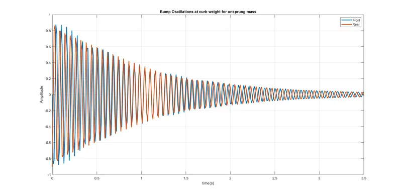
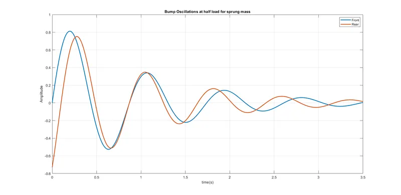
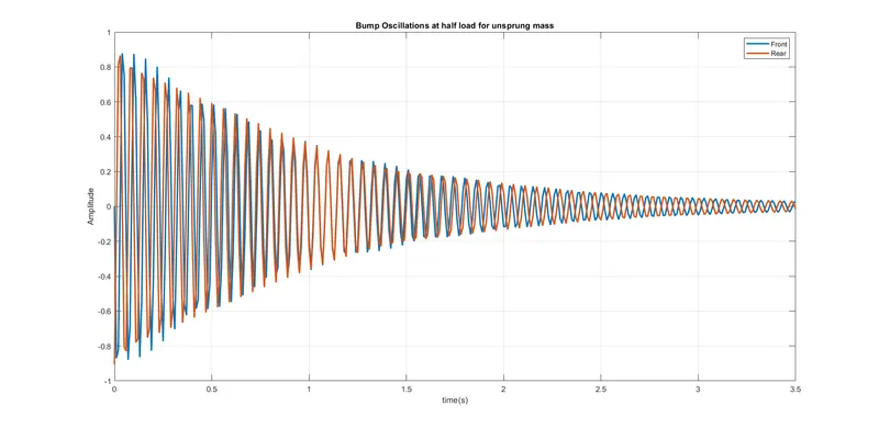
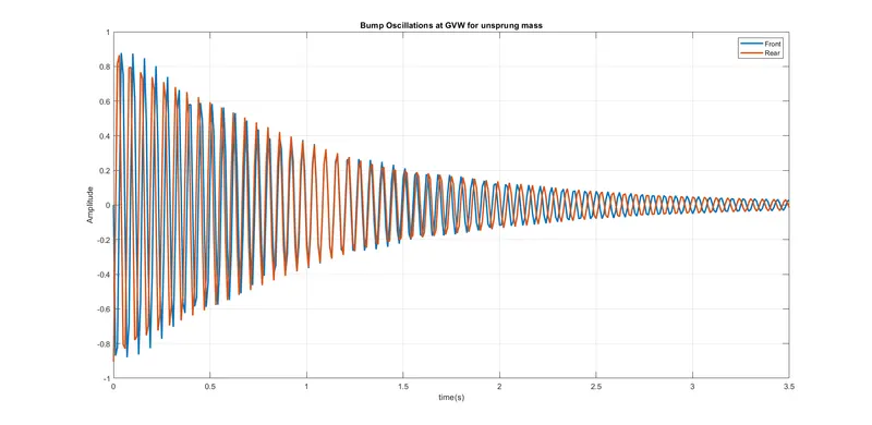
The MATLAB scripts and the sprung and unsprung bump oscillation plots for all 3 load conditions are given below.
a). Bump Oscillation at Curb Weight,
% Bump oscillation profile at curb weight.
clear all
close all
clc

% Corner sprung and unsprung weights.
Ms_front = 405; % Front sprung mass in Kg.
Ms_rear = 270;  % Rear sprung mass in Kg.
Mus_front = 45;     % Front unsprung mass in Kg.
Mus_rear = 30;      % Rear unsprung mass in Kg.

% Ride rate at curb weight.
Kr_front = 23.85; % In N/mm.
Kr_rear = 25.4;   % In N/mm.

% Wheel rate at curb weight.
Kw_front = 26.42; % In N/mm.
Kw_rear = 28.34;  % In N/mm.

%Tire rate at curb weight.
Kt = 245; % In N/mm for front and rear.

% Time lag between front and rear.
t_l = 0.1; % In seconds.

% Sprung mass frequencies at curb weight.
Fs_front = sqrt(Kr_front*1000/Ms_front)/(2*pi); %In Hz.
Fs_rear = sqrt(Kr_rear*1000/Ms_rear)/(2*pi);    % In Hz.

% Unsprung mass frequencies at curb weight.
Fus_front = sqrt((Kt+Kw_front)*1000)/(2*pi); % In Hz.
Fus_rear = sqrt((Kt+Kw_rear)*1000)/(2*pi);   % In Hz.

% Time step
t = [0:0.01:3.5]; % In seconds.

% Amplitude for sprung mass.
for i = 1:length(t)
    As_front(i) = exp(-t(i)).*sin(2*pi*Fs_front*t(i));
    As_rear(i) = exp(-t(i)).*sin(2*pi*Fs_rear*(t(i)-t_l));
end

% Amplitude for unsprung mass.
for j = 1:length(t)
    Aus_front(j) = exp(-t(j)).*sin(2*pi*Fus_front*t(j));
    Aus_rear(j) = exp(-t(j)).*sin(2*pi*Fus_rear*(t(j)-t_l));
end

% Plotting the graphs.
figure(1)
plot(t,As_front,"linewidth",2);
hold on;
plot(t,As_rear,"linewidth",2);
hold off;
grid on;
title("Bump Oscillations at curb weight for sprung mass");
xlabel("time(s)");
ylabel("Amplitude");
legend("Front","Rear");

figure(2)
plot(t,Aus_front,"linewidth",2);
hold on;
plot(t,Aus_rear,"linewidth",2);
hold off;
grid on;
title("Bump Oscillations at curb weight for unsprung mass");
xlabel("time(s)");
ylabel("Amplitude");
legend("Front","Rear");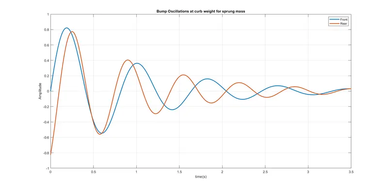
b). Bump Oscillation at Half Load,
% Bump oscillation profile at half load.
clear all
close all
clc

% Corner sprung and unsprung weights.
Ms_front = 456.875; % Front sprung mass in Kg.
Ms_rear = 380.625;  % Rear sprung mass in Kg.
Mus_front = 45;     % Front unsprung mass in Kg.
Mus_rear = 30;      % Rear unsprung mass in Kg.

% Ride rate at half load.
Kr_front = 23.85; % In N/mm.
Kr_rear = 25.4;   % In N/mm.

% Wheel rate at half load.
Kw_front = 26.42; % In N/mm.
Kw_rear = 28.34;  % In N/mm.

%Tire rate at half load.
Kt = 245; % In N/mm for front and rear.

% Time lag between front and rear.
t_l = 0.1; % In seconds.

% Sprung mass frequencies at half load.
Fs_front = sqrt(Kr_front*1000/Ms_front)/(2*pi); %In Hz.
Fs_rear = sqrt(Kr_rear*1000/Ms_rear)/(2*pi);    % In Hz.

% Unsprung mass frequencies at half load.
Fus_front = sqrt((Kt+Kw_front)*1000)/(2*pi); % In Hz.
Fus_rear = sqrt((Kt+Kw_rear)*1000)/(2*pi);   % In Hz.

% Time step
t = [0:0.01:3.5]; % In seconds.

% Amplitude for sprung mass.
for i = 1:length(t)
    As_front(i) = exp(-t(i)).*sin(2*pi*Fs_front*t(i));
    As_rear(i) = exp(-t(i)).*sin(2*pi*Fs_rear*(t(i)-t_l));
end

% Amplitude for unsprung mass.
for j = 1:length(t)
    Aus_front(j) = exp(-t(j)).*sin(2*pi*Fus_front*t(j));
    Aus_rear(j) = exp(-t(j)).*sin(2*pi*Fus_rear*(t(j)-t_l));
end

% Plotting the graphs.
figure(1)
plot(t,As_front,"linewidth",2);
hold on;
plot(t,As_rear,"linewidth",2);
hold off;
grid on;
title("Bump Oscillations at half load for sprung mass");
xlabel("time(s)");
ylabel("Amplitude");
legend("Front","Rear");

figure(2)
plot(t,Aus_front,"linewidth",2);
hold on;
plot(t,Aus_rear,"linewidth",2);
hold off;
grid on;
title("Bump Oscillations at half load for unsprung mass");
xlabel("time(s)");
ylabel("Amplitude");
legend("Front","Rear");
c). Bump Oscillation at GVW,
% Bump oscillation profile at Gross Vehicle Weight.
clear all
close all
clc

% Corner sprung and unsprung weights.
Ms_front = 475; % Front sprung mass in Kg.
Ms_rear = 450;  % Rear sprung mass in Kg.
Mus_front = 45;     % Front unsprung mass in Kg.
Mus_rear = 30;      % Rear unsprung mass in Kg.

% Ride rate at GVW.
Kr_front = 23.85; % In N/mm.
Kr_rear = 25.4;   % In N/mm.

% Wheel rate at GVW.
Kw_front = 26.42; % In N/mm.
Kw_rear = 28.34;  % In N/mm.

%Tire rate at GVW.
Kt = 245; % In N/mm for front and rear.

% Time lag between front and rear.
t_l = 0.1; % In seconds.

% Sprung mass frequencies at GVW.
Fs_front = sqrt(Kr_front*1000/Ms_front)/(2*pi); %In Hz.
Fs_rear = sqrt(Kr_rear*1000/Ms_rear)/(2*pi);    % In Hz.

% Unsprung mass frequencies at GVW.
Fus_front = sqrt((Kt+Kw_front)*1000)/(2*pi); % In Hz.
Fus_rear = sqrt((Kt+Kw_rear)*1000)/(2*pi);   % In Hz.

% Time step
t = [0:0.01:3.5]; % In seconds.

% Amplitude for sprung mass.
for i = 1:length(t)
    As_front(i) = exp(-t(i)).*sin(2*pi*Fs_front*t(i));
    As_rear(i) = exp(-t(i)).*sin(2*pi*Fs_rear*(t(i)-t_l));
end

% Amplitude for unsprung mass.
for j = 1:length(t)
    Aus_front(j) = exp(-t(j)).*sin(2*pi*Fus_front*t(j));
    Aus_rear(j) = exp(-t(j)).*sin(2*pi*Fus_rear*(t(j)-t_l));
end

% Plotting the graphs.
figure(1)
plot(t,As_front,"linewidth",2);
hold on;
plot(t,As_rear,"linewidth",2);
hold off;
grid on;
title("Bump Oscillations at GVW for sprung mass");
xlabel("time(s)");
ylabel("Amplitude");
legend("Front","Rear");

figure(2)
plot(t,Aus_front,"linewidth",2);
hold on;
plot(t,Aus_rear,"linewidth",2);
hold off;
grid on;
title("Bump Oscillations at GVW for unsprung mass");
xlabel("time(s)");
ylabel("Amplitude");
legend("Front","Rear");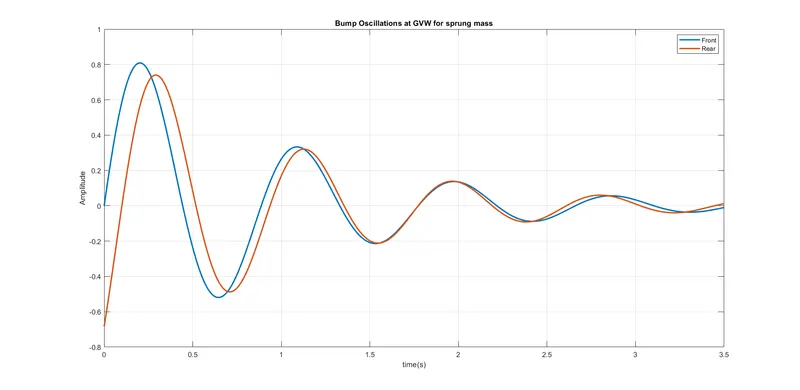
Result,
From the plots it can be observed that the bump oscillations are out of phase at curb weight and are in phase at gross vehicle weight.
CONCLUSION :-
- The spring parameters for all 3 load conditions are calculated.
- The bump oscillation profiles for all 3 load conditions are plotted using MATLAB.