Week 9 - FVM Literature Review
Finite Volume Methods
Finite volume methods (FVM) are a great discretization key to solve physical behaviors in spots where the mesh geometry varies from one point to another one. The best advantage of Finite Volume Methods (FVM) is this one can solve irregular meshes using the Gauss theorem and dividing the mesh in small volume cells; Finite Difference Methods (FDM) are typically used in physical problems where the geometry is regular and concentric as a square CAD solid or phenomenas where the wheater is the only one who is affecting a determined spot. FVM has more applications in the PDE solutions, due to its easily way to fit itself to different environments, and it can be seen used in analysis where the solid CAD can be tapered or geometries analysis as the flow behavior over an aircraft airfoil, while FDM does not achieve to fit itself in this kind of analyses. However, FDM is often used in astrologic due to this method can increase its accurate degree without affect the mesh, something the FVM shows some lacks.
Let's get do an FVM example: It is going to be calculated the behavior of the 1D-Steady Diffusivity behavior along a tapered tank which has the following shape:
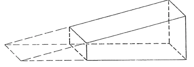
Due to the irregular shape of the tank, diffusivity equation can be present some issues if this one is solved using FDM, so, 1D-Steady diffusivity equation is represented as:
`alpha(partial^2u)/(partialx^2)=0`
This can also be written as:
`(partial)/(partialx)alpha(partialu)/(partialx)+S=0`
Where S is equal to the source term or the term which the equation is going to be linearized with. Now, the well known grid points that were normally used in FDM are going to be closed by a finite volume as is shown in the following image. W could be i=1, P could be i=2 and etc. This division will depend on the number of nodes the length has been divided.
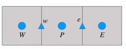
These points will be located at the center of the volume shape. After the whole points have been closed, the net step is to multiplicate the diffusivity equation by the differential volume integer and integrate the equation:
`int_e^w((partial)/(partialx)alpha(partialu)/(partialx)+S)dV=0`
Looking at the volume division picture, the bottom and top line will be dx and the surface area that is located looking the volume at the left side will be the `dy*dz` area; this area is expressed as A in the equation. The equation will fit as:
`Aalpha((partialu)/(partialx))_e^w+int_e^wSdV=0`
Finally, calculating the first term as a function of w and e and, using Taylor series approximation to find the partial terms, the previous equation is given as:
`alphaA((u_e-u_p)/(Deltax))-alphaA((u_p-u_w)/(Deltax))+overline(S)dV=0`
The two first terms in the equation are known as flux terms, the third one is known as the source term. If `overline(S)` is a function of u, it will be obtained the equation:
`S_u+S_pu_p`
To calculate the value of the face cells it is necessary to use interpolation schemes, which define the terms that are interpolated values from cell centers to face centers. These are primarily used in the calculation of velocity to the face centers for the calculation of flux. There are different interpolation schemes, but the most known are:
1. Upwind Interpolation Scheme
The upwind interpolation for approximating the value of a variable 'f' at the east face of the control volume is given as below. We want approximation at the eastern face 'e':
`{(f_P if (v*n_e)>0),(f_E if(v*n_e)<0):}`
Where (v.n)e is the velocity component at point e in x direction.
2. Linear Interpolation Scheme
The linear intepolation is equivalent to the use of the central difference formula of the first order derivative and hence it is also called as Central Difference Scheme(CDS). It is second order accurate whose accuracy is very good but we might have one small problem for advection dominated situations, that this scheme may produce oscillatory solutions, This scheme leads to simple approximation for evaluation of gradients required for evaluation of diffusive fluxes:
`f_e=f_E*lamda_e+f_P*(1-lamda_e)`
Where `lamda_e=(x_e-x_p)/(x_E-x_P)`
Those two are some examples of interpolation schemes used for calculating the face terms. Also, in high interpolations the flux limiters are an important thing due to the main idea behind the construction of flux limiter schemes is to limit the spatial derivatives to realistic values The main purpose of flux limiter is to keep the values bounded at the cell faces. Flux limiter don't let the solution value to overshoot. Considering a 1D semi Discrete scheme:
`(du_i)/dt+1/(Deltax_i)[F_(u_i+1/2)-F_(u_i-1/2)]=0`
Represents the edge fluxes for the ith cell can be represented by low and high resolution schemes then the flux limiter can switch between these schemes depending upon the gradients close to the particular cell:
`F_(u_i+1/2)=f_(i+1/2)^(low)-phi(r_i)(f_(i+1/2)^(low)-f_(i+1/2)^(high))`
`F_(u_i-1/2)=f_(i-1/2)^(low)-phi(r_i)(f_(i-1/2)^(low)-f_(i-1/2)^(high))`
`r_i`represents the ratio successive gradients on the resolution mesh:
`r_i=(u_i-u_(i-1))/(u_(i+1)-u_i)`
REFERENCES
https://www.youtube.com/watch?v=4n3DPwcoy4E
https://engineeringlibrary.org/reference/beam-torsion-air-force-stress-manual