Week 9- Unsteady moving zones Approach

Unsteady Moving Zones Approach

AIM

The following project is carried out in order to use a meshing model concept well-known as moving zones; This method is very useful for simulating flows that are enclosed into a case, while the flow is displaced for another solid component that can move rotationally or translationally into the case.

In this project, three different meshes of a generic turbomachinery are provided and they must be assembled; then, to compare the two different methods for solving the flow behavior, it will be performed two different simulations, with steady and transient solvers. Finally, the results obtained at each simulation will be plotted and analyzed, to determine the accuracy of each method.

OBJECTIVES

Assemble the domains of generic turbomachinery provided by the project statements and carry out the required actions to refine and fit each mesh.

Simulate the flow behavior into the generic turbomachinery, by using steady and unsteady solver methods, and taking into account that the airfoils settled into the second domain must rotate with a determined angular velocity.

Analyze the results obtained from each solver method and compare them to determine whether the simulations have obtained the same results.

ENGINEERING DEVELOPMENT

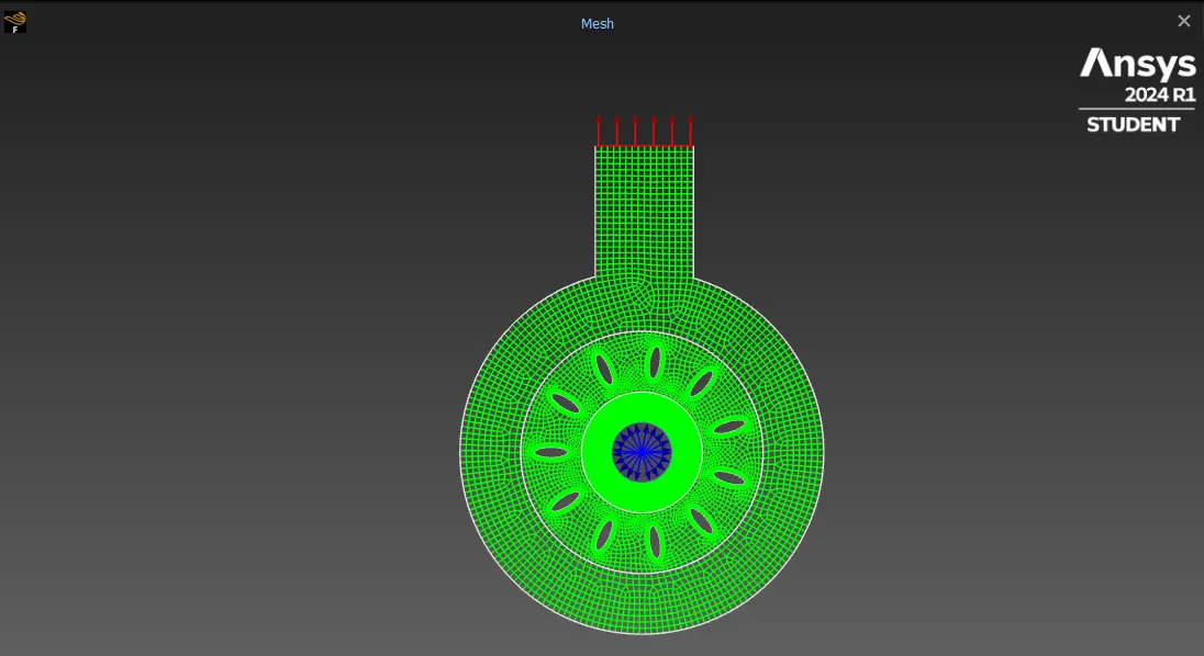
The first step is to assemble the domains provided by the project statements; to do that, it is only necessary to update the first domain, then, using the append tool located on the domain icon, the second and third domains are updated too. The mesh result should look like the image shown below.

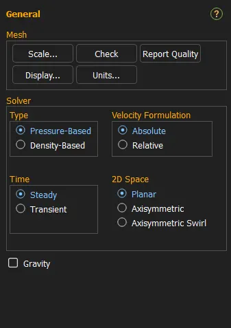
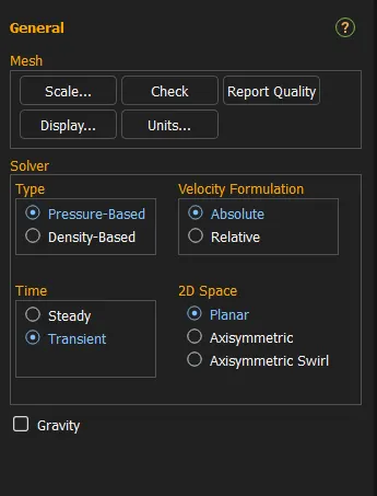
In addition, the solver type is set according to the next two images, depending on the type of simulation that it is going to carry out.

Steady type solver

Transient type solver

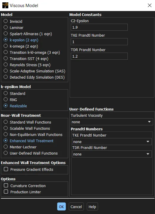
Now, to set the turbulence model, the literature advises that the `k-epsilon` model is more approximated to get accurate results. Thus, the turbulence model chosen is also set with a Realizable model and the wall is put with an enhanced wall treatment.

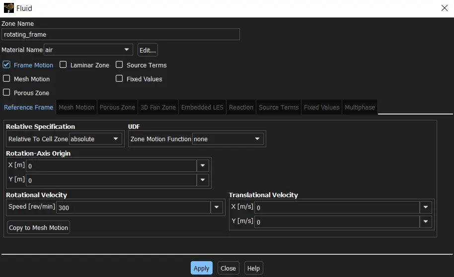
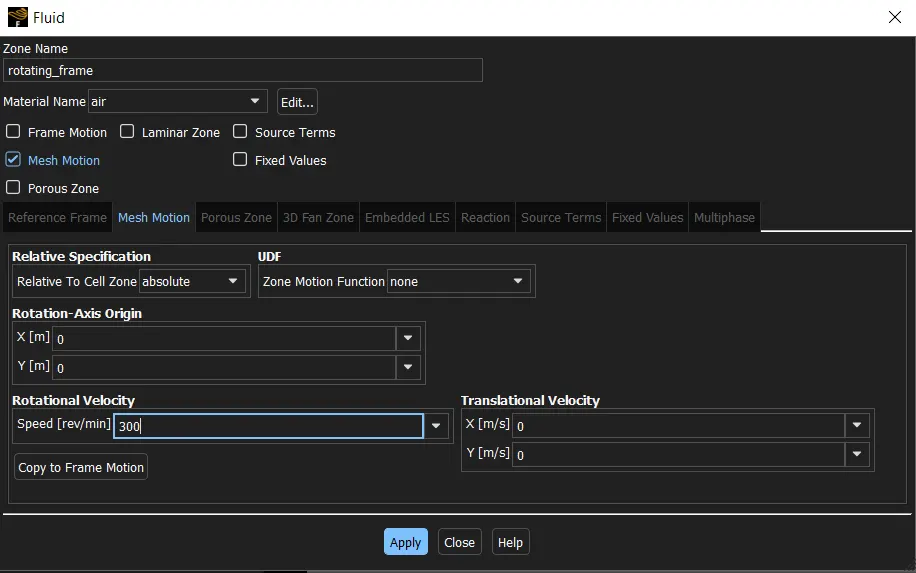
Likewise, the cell zone conditions must be set according to the next two images, taking into account that the moving zone method for steady simulations is carried out with the frame motion and, with the mesh motion for unsteady solutions. The angular velocity at which the airfoils will rotate, is equal to 300 rpm.

Steady type solver

Transient type solver

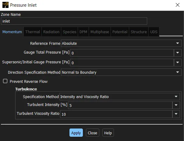
The next step is to enter the boundary conditions of each turbomachinery part, taking the inlet as a pressure inlet.

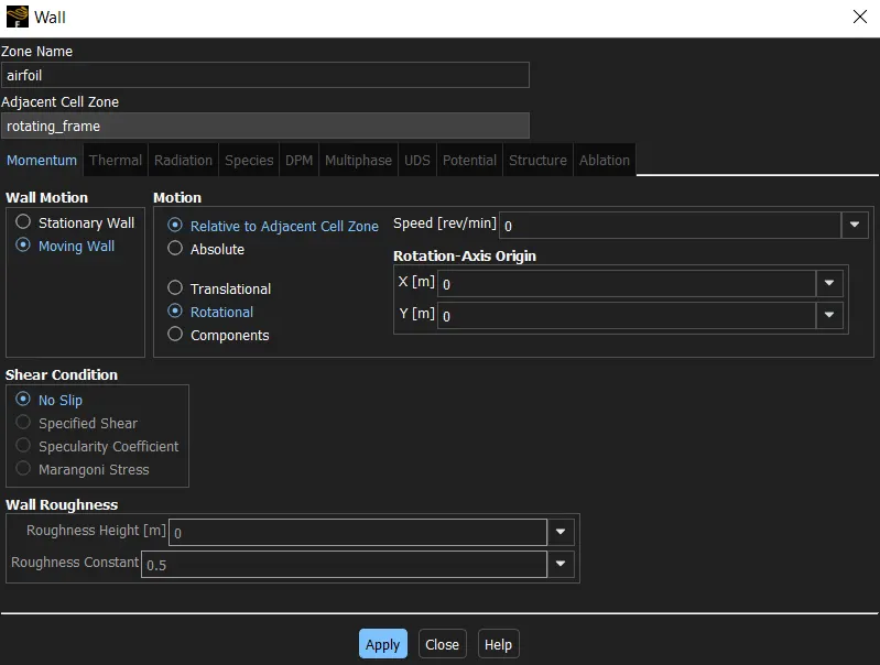
In the same way, the airfoils must be set as moving walls with a rotational movement.

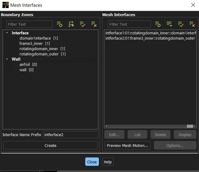
Some surfaces must be joined such that the cells interact together and the program does not take these sections as walls; these surfaces are the surfaces where two domains are connected, therefore the surfaces that are interlaced, are connected by using the mesh interfaces tool.

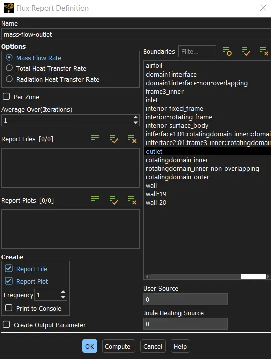
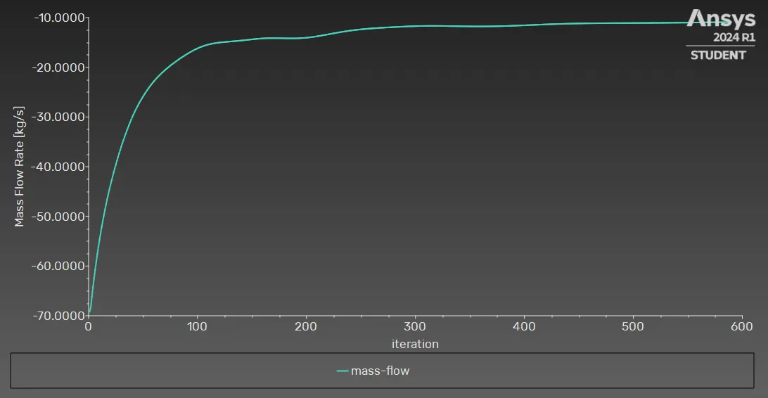
Once the physical features are correctly set, it can be selected the parameters that may be convenient to obtain; in this case, the mass flow rate at the outlet section is only selected.

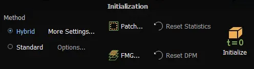
Before starting the simulation, the initialization is performed by using the hybrid method:

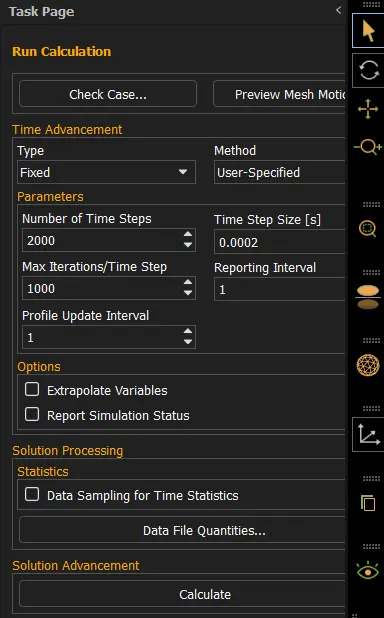
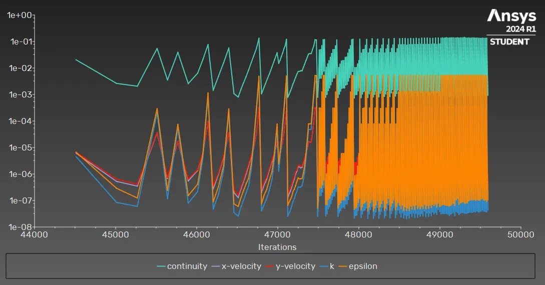
Furthermore, the number of iterations is taken in order to get a convergence solution before all number of iterations have been completed.

Steady type solver

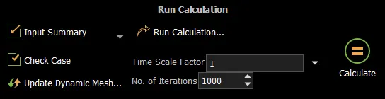
Transient type solver

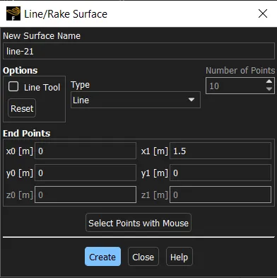
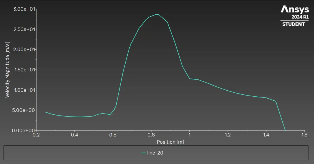
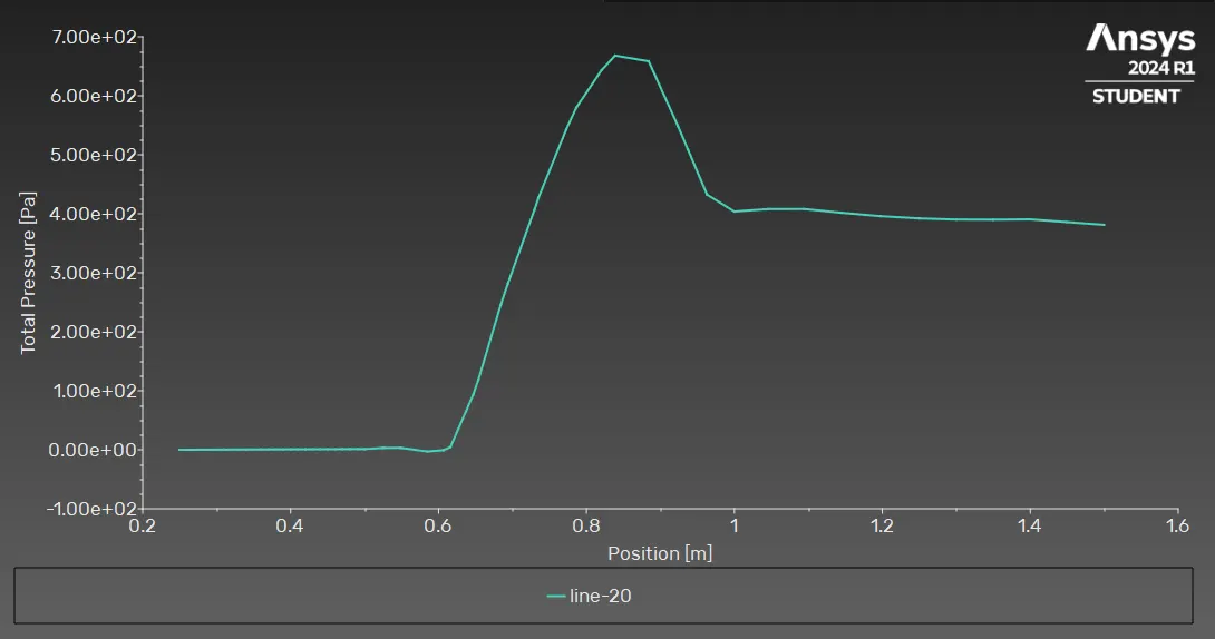
Finally, to get pressure and velocity results along a certain distance from the diameter center to the external case, it can be created a line that takes those values.

RESULTS

The results obtained for each type of simulation are shown in the following images:

Steady-type solver results

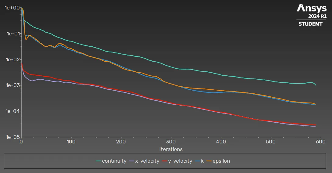
• Simulation convergence

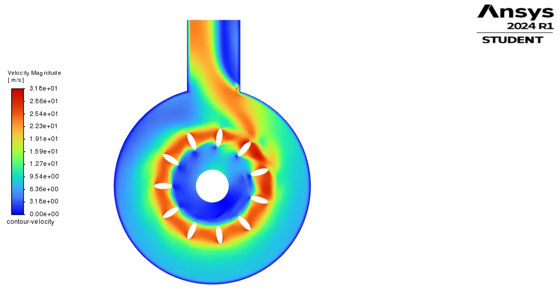
• Velocity profile

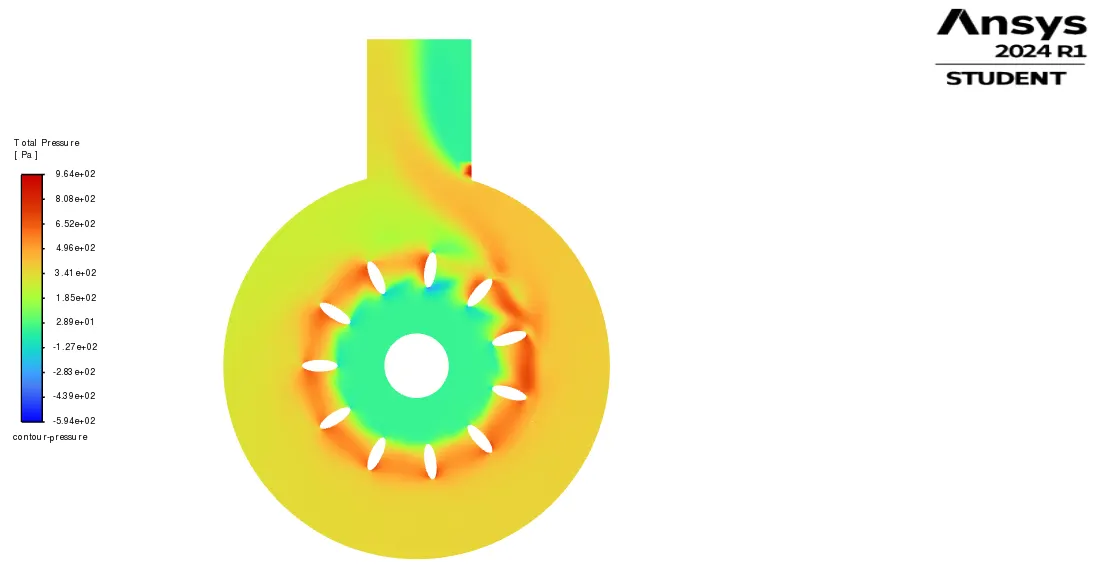
• Total pressure profile

• Mass flow rate

• Velocity magnitude along the X positive axis

• Total pressure magnitude along the X positive axis

Transient-type solver results

• Simulation convergence

• Velocity profile

• Total pressure profile

• Mass flow rate

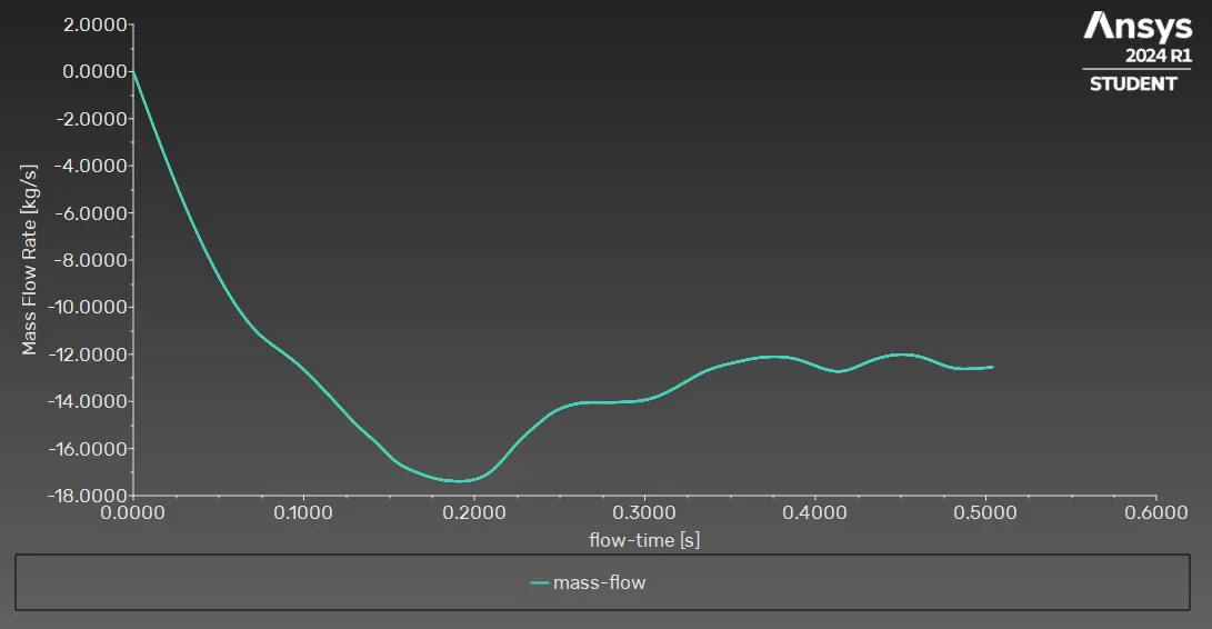
The average mass flow rate value that the flow is leaving the domain with, is shown in the next table for each result obtained:

Solver type	Mass Flow Rate (Kg/s)	Error percentage (%)
Steady	10.913	4.54
Transient	11.408

The percentage error between the two simulations is below 5%, however, it should be considered too high, taking into account that the simulation is only varying in solver type. The velocity and pressure profiles also get the same error.

CONCLUSIONS

To get more accurate results, the number of iterations per step in an unsteady solver should be greater than the one that was used in the current project.

REFERENCES

https://www.researchgate.net/publication/361004841_Turbulence_Considerations_in_Turbomachinery