Week 3.5 - Deriving 4th order approximation of a 2nd order derivative using Taylor Table method

Fourth Order Approximation for 2nd Order Analysis Report

1. AIM:

The main purpose of this report is to analyze the equation behavior for a function derivated twice, using 4th order taylor series; firstly, it will be used the taylor tables, in order to find the general equation for centered, skewed right-sided and skewed left-sided difference approximations and, using the MATLAB software, it will sort and find the constant coefficients which are along with each segment of each equation. Secondly, once the equations were found, it is necessary to perform some functions that solve an analytical 2nd derivative function given by the report exercise in an approximated way. Finally, these equations obtained will be compared with the analytical function, analyzing the functions behavior and the error that exists between the approximation equation and the analytical derivate.

2. OBJECTIVES OF THE PROJECT:

• Determine the 4th order approximation equation by means of Taylor series.
• Perform a code which sort each approximation equation, using MATLAB software.
• Analyze the results obtained on the plots and explain briefly the reason of this behavior.

3. PROJECT DEVELOPMENT:

Regarding with the report statements, it is known that the approximation equations can be solved easily with, due to the taylor tables provide enough information about the Taylor series coefficients when the number of analysis nodes are increased; the increment of the nodes chosen serves for solving and finding the equation which will use to find the approximate value of whatever derivative function. In this case, the Taylor equation will be solved in order to take the 4th order approximation and it will be analyzed the absolute error that the equation has, depending wether it is approximate from the center, skewed right sided or, skewed left sided. To do this, firstly the main equation must be defined and, this one can be defined if the number of nodes that must be taken are known; The way to know the number of nodes is:

• Centered difference approximation

The order of accuracy P = Number of nodes in the stencil N - order of derivative Q + 1

• Skewed Left/Right-sided difference approximation

The order of accuracy P = Number of nodes in the stencil N - order of derivative Q

As it was described above, the order of derivative is going to be two and the equation order is going to be by 4th order, and solving the equations named, the number of nodes to calculate the approximation centered will be 5 and 6 for skewed Left/Right-sided. So, the equations could be described as the following form:

• Centered difference approximation equation

`(partial^2f)/(partialx^2)=a*f(i-2)+b*f(i-1)+c*f(i)+d*f(i+1)+e*f(i+2)`

• Skewed Right-sided difference approximation equation

`(partial^2f)/(partialx^2)=a*f(i)+b*f(i+1)+c*f(i+2)+d*f(i+3)+e*f(i+4)+f*f(i+5)`

• Skewed Left-sided difference approximation equation

`(partial^2f)/(partialx^2)=a*f(i-5)+b*f(i-4)+c*f(i-3)+d*f(i-2)+e*f(i-1)+f*f(i)`

On each equation it can be seen some letters which represent the constant coefficient, which could accompain the term as it was seen in the equations for first derivative function. Taylor table is an arrangement of the coefficients that are along with each taylor equation term, when the equation is modified due to the next x value taken was once greater or even more. If the function is represented as "f(i+2)", that means the next step that will be taken from the x axis will be `x+2Deltax`; in general, the equation will analyze as:

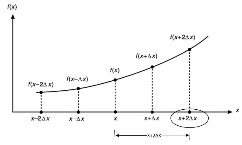
Likewise, the equation in each term can be written like this:

`f(i+n)=f(i)+O(n)`

Where O(n) is called the truncation error and f(i) is the original function. Taking all mentioned before into account, it can be described the equation of each term as:

`f(i+n)=f(i)+(nDeltax)/(1!)f'(i)+(nDeltax)^2/(2!)f''(i)+(nDeltax)^3/(3!)f'''(i)+...+(nDeltax)^n/(n!)f^n(i)`

or

`f(i-n)=f(i)-(nDeltax)/(1!)f'(i)+(nDeltax)^2/(2!)f''(i)-(nDeltax)^3/(3!)f'''(i)+...+(nDeltax)^n/(n!)f^n(i)`

Likewise, the Taylor tables is written as:

	`f(i)`	`(partialf(i))/(partialx)`	`(partialf^2(i))/(partialx^2)`	`(partialf^3(i))/(partialx^3)`	`(partialf^4(i))/(partialx^4)`	`(partialf^5(i))/(partialx^5)`	`(partialf^6(i))/(partialx^6)`	. . .	`(partialf^n(i))/(partialx^n)`
`f(i-5)`	1	-`(5Deltax)/(1!)`	`(5Deltax)^2/(2!)`	-`(5Deltax)^3/(3!)`	`(5Deltax)^4/(4!)`	-`(5Deltax)^5/(5!)`	`(5Deltax)^6/(6!)`		`(5Deltax)^n/(n!)`
`f(i-4)`	1	-`(4Deltax)/(1!)`	`(4Deltax)^2/(2!)`	-`(4Deltax)^3/(3!)`	`(4Deltax)^4/(4!)`	-`(4Deltax)^5/(5!)`	`(4Deltax)^6/(6!)`		`(4Deltax)^n/(n!)`
`f(i-3)`	1	-`(3Deltax)/(1!)`	`(3Deltax)^2/(2!)`	-`(3Deltax)^3/(3!)`	`(3Deltax)^4/(4!)`	-`(3Deltax)^5/(5!)`	`(3Deltax)^6/(6!)`		`(3Deltax)^n/(n!)`
`f(i-2)`	1	-`(2Deltax)/(1!)`	`(2Deltax)^2/(2!)`	-`(2Deltax)^3/(3!)`	`(2Deltax)^4/(4!)`	-`(2Deltax)^5/(5!)`	`(2Deltax)^6/(6!)`		`(2Deltax)^n/(n!)`
`f(i-1)`	1	-`(Deltax)/(1!)`	`(Deltax)^2/(2!)`	-`(Deltax)^3/(3!)`	`(Deltax)^4/(4!)`	-`(Deltax)^5/(5!)`	`(Deltax)^6/(6!)`		`(Deltax)^n/(n!)`
`f(i)`	1	0	0	0	0	0	0		0
`f(i+1)`	1	`(Deltax)/(1!)`	`(Deltax)^2/(2!)`	`(Deltax)^3/(3!)`	`(Deltax)^4/(4!)`	`(Deltax)^5/(5!)`	`(Deltax)^6/(6!)`		`(Deltax)^n/(n!)`
`f(i+2)`	1	`(2Deltax)/(1!)`	`(2Deltax)^2/(2!)`	`(2Deltax)^3/(3!)`	`(2Deltax)^4/(4!)`	`(2Deltax)^5/(5!)`	`(2Deltax)^6/(6!)`		`(2Deltax)^n/(n!)`
`f(i+3)`	1	`(3Deltax)/(1!)`	`(3Deltax)^2/(2!)`	`(3Deltax)^3/(3!)`	`(3Deltax)^4/(4!)`	`(3Deltax)^5/(5!)`	`(3Deltax)^6/(6!)`		`(3Deltax)^n/(n!)`
`f(i+4)`	1	`(4Deltax)/(1!)`	`(4Deltax)^2/(2!)`	`(4Deltax)^3/(3!)`	`(4Deltax)^4/(4!)`	`(4Deltax)^5/(5!)`	`(4Deltax)^6/(6!)`		`(4Deltax)^n/(n!)`
`f(i+5)`	1	`(5Deltax)/(1!)`	`(5Deltax)^2/(2!)`	`(5Deltax)^3/(3!)`	`(5Deltax)^4/(4!)`	`(5Deltax)^5/(5!)`	`(5Deltax)^6/(6!)`		`(5Deltax)^n/(n!)`

• Centered difference approximation equation:

Taking each term defined above and matching each term equation regarding their derivate order, the equations that will find out the constant coefficients are:

`a+b+c+d+e=0`

`-2a-b+d+2e=0`

`2a+b/2+d/2+2e=1`

`-4/3a-1/6b+1/6d+4/3e=0`

`2/3a+1/24b+1/24d+2/3e=0`

All these equations are replaced on a 5x5 matrix and using MATLAB software, these are solved; the matrix is defined as:

`[[1,1,1,1,1],[-2,-1,0,1,1],[2,1/2,0,1/2,2],[-4/3,-1/6,0,1/6,4/3],[2/3,1/24,0,1/24,2/3]][[a],[b],[c],[d],[e]]=[[0],[0],[1],[0],[0]]`

It must take into account the whole equations are divided by `Deltax^2`. Solving the matrix on MATLAB, the coefficient values are:

`a=-1/12`

`b=4/3`

`c=-5/2`

`d=4/3`

`a=-1/12`

-MATLAB Code:

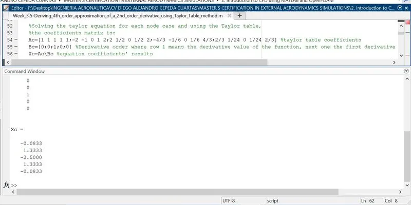
Finally, solving a little the equation and decreasing terms, the general centered difference 4th order approximation equation is:

`(partial^2f)/(partialx^2)=(-f(i-2)+16f(i-1)-30f(i)+16f(i+1)-f(i+2))/(12Deltax^2)`

Getting a truncation error of `O(Deltax^4)`; this truncation error has the same order level for right and left sided difference approximation.

• Skewed right-sided difference approximation equation:

In this case, it will be taken the values from x until `x+5Deltax` and, knowing there are six terms into the equation, the equations to find the coefficients are defined as the following form:

`a+b+c+d+e+f=0`

`b+2c+3d+4e+5f=0`

`b/2+2c+9/2d+8e+25/2f=1`

`b/6+4/3c+9/2d+32/3e+125/6f=0`

`b/24+2/3c+27/8d+32/3e+625/4f=0`

`b/120+4/15c+81/40d+128/15e+625/24f=0`

As it was performed for finding out the centered difference equation, this coefficients will be added on a 6x6 matrix and also, they will be solved on MATLAB. The matrix and results are shown respectively:

- Matrix

`[[1,1,1,1,1,1],[0,1,2,3,4,5],[0,1/2,2,9/2,8,25/2],[0,1/6,4/3,9/2,32/3,125/6],[0,1/24,2/3,27/8,32/3,625/24],[0,1/120,4/15,81/40,128/15,625/24]][[a],[b],[c],[d],[e],[f]]=[[0],[0],[1],[0],[0],[0]]`

-Coefficient Results

`a=15/4`

`b=-77/4`

`c=107/4`

`d=-13`

`e=61/12`

`f=-5/6`

-MATLAB code

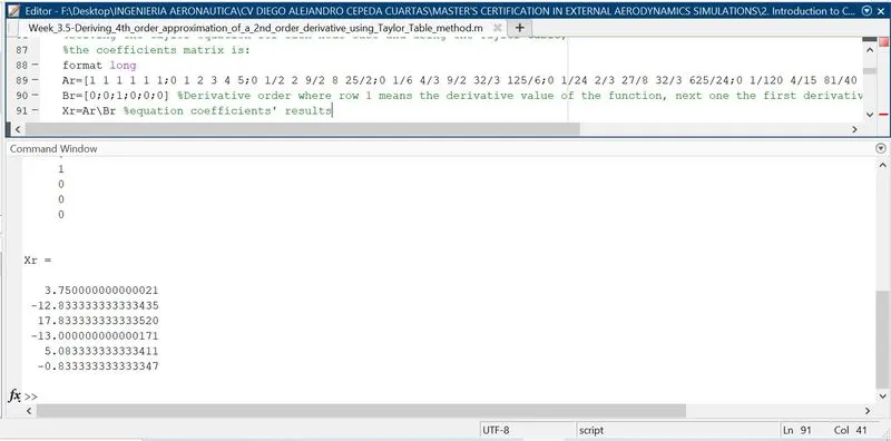
In this case, all coefficients are also divided by `Deltax^2`; The equation for 4th order Skewed right-sided difference approximation can be solved and adjusted, getting the following equation:

`(partial^2f)/(partialx^2)=(45f(i)-154f(i+1)+214f(i+2)-156f(i+3)+61f(i+4)-10f(i+5))/(12Deltax^2)`

• Skewed left-sided difference approximation equation:

The missing equation that have to be found is the equation for 4th order skewed left-sided difference approximation equation. To do this, it is necessary to be clear the equation is as similar as the previous equation, but the values begin from i to i-5, due to that, the equations to find the coefficients are:

`a+b+c+d+e+f=0`

`-5a-4b-3c-2d-5e=0`

`25/2a+8b+9/2c+2d+1/2e=1`

`-125/6a-32/3b-9/2c-4/3d-e/6=0`

`625/4a+32/3b+27/8c+2/3d+1/24e=0`

`-625/24a-128/15b-81/40c-4/15d-1/120e=0`

And the matrix and results are given as the following form:

- Matrix

`[[1,1,1,1,1,1],[-5,-4,-3,-2,-1,0],[25/2,8,9/2,2,1/2,0],[-125/6,-32/3,-9/2,-4/3,-1/6,0],[625/24,32/3,27/8,2/3,1/24,0],[-625/24,-128/15,-81/40,-4/15,-1/120,0]][[a],[b],[c],[d],[e],[f]]=[[0],[0],[1],[0],[0],[0]]`

-Coefficient Results

`a=-5/6`

`b=61/12`

`c=-13`

`d=107/6`

`e=-77/6`

`f=15/4`

-MATLAB code

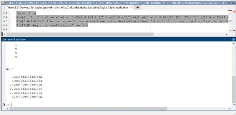
Results divided by `Deltax^2` like the other two equations previously described. At the same way the previous equation could be adjusted, the equation for 4th order skewed left-sided difference approximation is also solved and adjusted, getting the formula:

`(partial^2f)/(partialx^2)=(-10f(i-5)+61f(i-4)-156f(i-3)+214f(i-2)-154f(i-1)-45f(i))/(12Deltax^2)`

**To catch up with the code exposed on the pictures, do not doubt to watch the files attached below of this report**

All these equations have to be evaluated, entering the analytical equation; the analytical equation that will be taken in this analysis is:

`f(x)=e^xcos(x)`

Derivating the analytical function twice, it is obtained the formula:

`f'(x)=e^xcos(x)-e^xsin(x)` - First derivative

`f''(x)=-2e^xsin(x)` - Second derivative

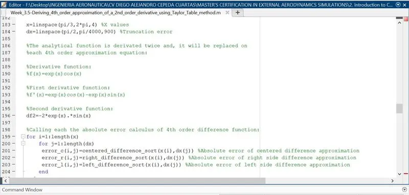
And the equation obtained is put on the approximation equations. MATLAB is used again in order to analyze and dtermine the equations behavior as when the X value on the equation change as when the truncation value (DX) is decreased. The main code contains the matrix showed above and, likewise, this file was used to call the functions performed to analyze the absolute error in each equation approximation and how the function looks like when the truncation error is too high and too low.

The fisrt part of the code was already shown, this part solves the matrix to get the constant coefficient values. The second part of the main code calls the functions performed to analyze the absolute error for each approximation equation, using a for loop, and the truncation error values are varied from `Deltax=pi/4` to `Deltax=pi/4000`, dividing their length in 900 parts. All the equations are evaluted changing the X value from `pi/3` to `2pi`, because of the absolute error could increase or decrease regarding the X value analyzed. It was taken only 4 different values between `pi/3 and 2pi`.

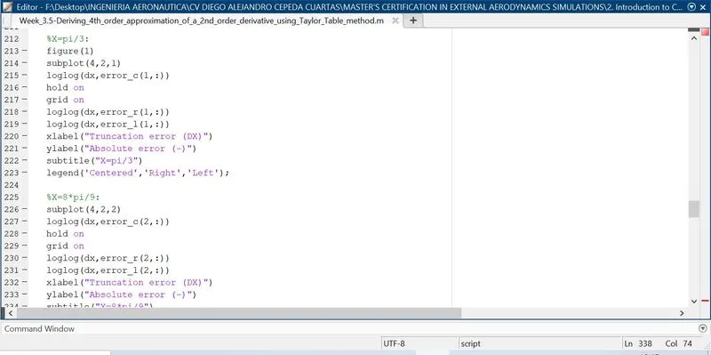
The plot of the absolute error behavior regarding the truncation error change is shown in the following picture. Due to the size of the plot code, it is only shown the code structure when the x value is equal to `pi/3` and `(8pi)/9` for, but is the same code for the next two x values.

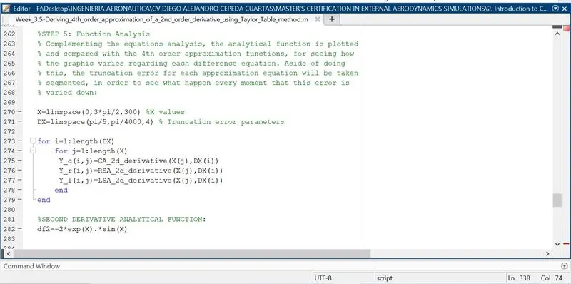
The third part of the main code is about how the function plot looks like when the truncation error is less than the last of this one. This part was developed in order to show how the error calculated on the second part affects the function plot behavior regarding the analytical function.

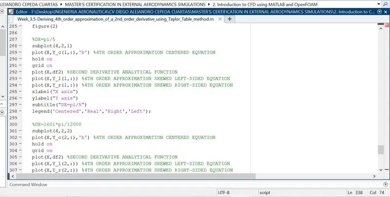
Aside of divide the X value in 300 parts of its length, the plots are also analyzed in different truncation error values and it is plotted each function behavior regarding a specific truncation error value taken. The next picture shows the code trsucture used for plotting the functions, but it is only show the code for `DX=pi/5` and `DX=(1601pi)/12000`.

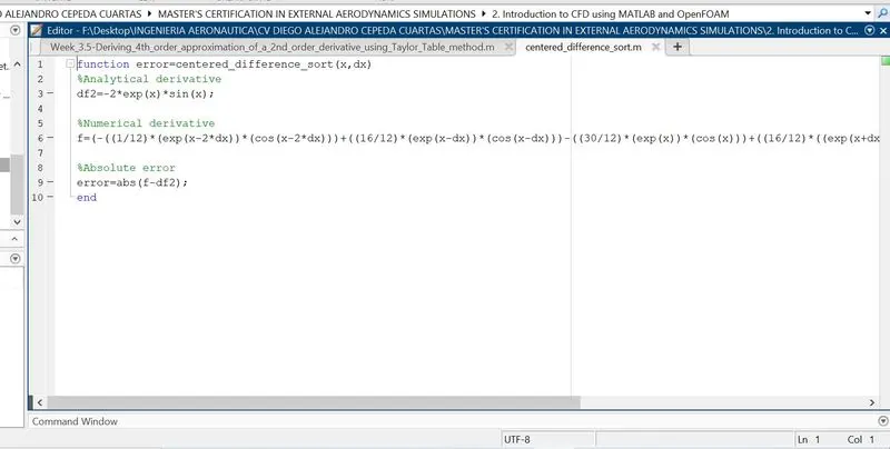
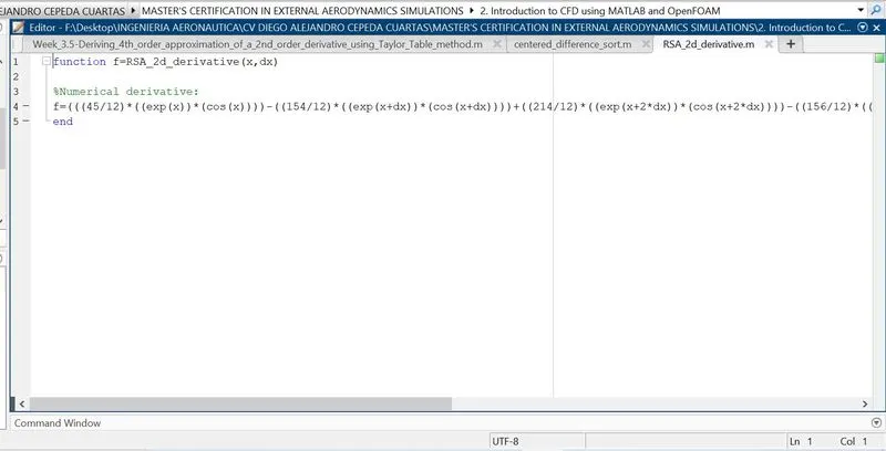
As regards to the functions called by the for loop, each function code file has the approximation equation depending of the difference position assigned (centered, left or right sided). In the next two pictures can be seen the function to calculate the absolute error and, the function to throw the f(x)'s values for plotting the functions behavior.

• MATLAB code of Absolute error function - centered difference approximation

• MATLAB code of Y values function - skewed right-sided difference approximation

4. RESULTS:

Running up the code of the second part, the sesult abtained is the plots shown below:

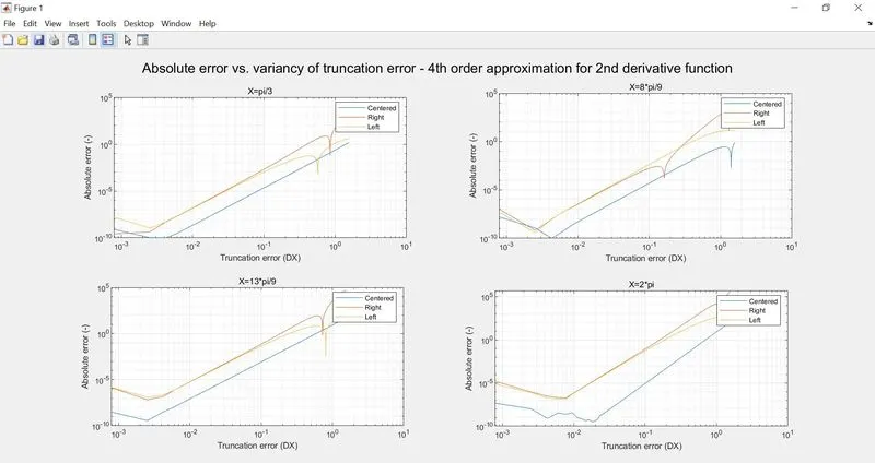
It can be noticed the absolute error is less for centered difference than the two others and, furthermore, regarding the x value increases, the absolute error will tend to be unstable in a faster way than the small values; this is deducted because of, if the lower peek in each line is analyzed, it can be determined the peek is greater than the previous x value analyzed. However, the centered difference behavior tends to keep more constant than left and right difference behavior.

The absolute error affects the function behavior as it was described above, this argument is noticed once the third part of the code is ran up and the following plot is obtained. The plot shows that, depending of the x value and the truncation value taken to carry out the analysis, the approximation functions move away from the real function.

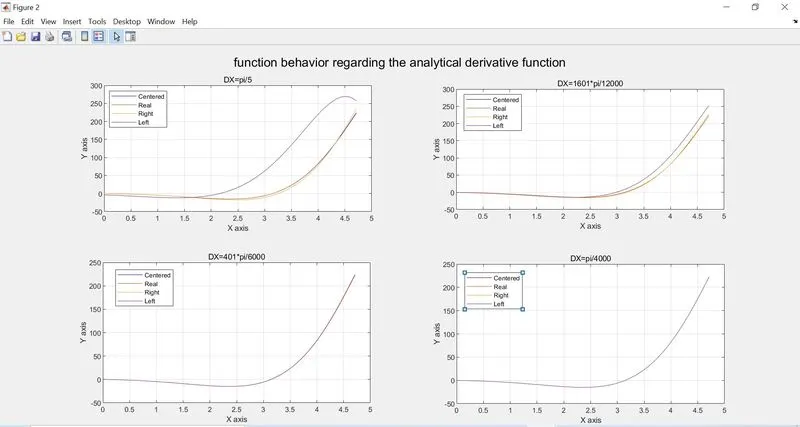
On the first plot, left difference is too far from the real function, even from the other two approximations, due to the truncation error is too high and, likewise, the absolute error but, if the last plot is analyzed, it can be seen the approximations tends to adjust until look like the real function, because of the truncation error is lower but not too much lower for unstabilizing the function behavior.

All MATLAB code files are attached ta the end of this report. However the main code and one of each code for absolute error and function behavior are attached below:

Main MATLAB code:

%Weeek 3.5 - Deriving 4th order approximation of a 2nd order derivative using Taylor Table method
% Diego Alejandro Cepeda Cuartas

%Derive the following 4th order approximations of the second-order derivative. 
%1. Central difference
%2. Skewed right-sided difference
%3. Skewed left-sided difference

%After deriving these schemes, prove that your skewed schemes are fourth-order accurate 
%i.e the thumb rule given in HINT (ii). 
%Once you have done this, write a program in Matlab to evaluate the second-order derivative 
%of the analytical function exp(x)*cos(x) and compare it with the 3 numerical approximations 
%that you have derived.

%Provide a plot that compares the absolute error between the above-mentioned schemes

%In your own words, describe why a skewed scheme is useful? What can a skewed scheme 
%do that a CD scheme cannot?

%HINT :
%i) The order of accuracy P = Number of nodes in the stencil N - order of derivative Q + 1 
%for symmetric/central schemes

%ii) The order of accuracy P = Number of nodes in the stencil N - order of derivative Q   
%for one-sided/skewed schemes 

%iii) Solve the system of equations using the matrix inversion method in Matlab to obtain the 
%taylor table coefficients and use them directly in the numerical approximation statements to avoid 
%input errors. 

%SOLUTION:
%CODE:
clear all
clc
%1. Centered Difference: 
%STEP 1: Finding the number of nodes

%According to the hint part shown below, the number of accuracy order is given 
%by: P=N-Q+1

%Where P:Number of Accuracy Order; Q:Number of Derivative Order; N: Number
%of nodes

%So, the number of nodes should be: N=P+Q-1

%In this case Q=2 and P=4. The number of nodes should be N=5.

%STEP 2: Calculate the coefficients:
%It will take the number of nodes as: 
%(df/dx)^2=a*f(i-2)+b*f(i-1)+c*f(i)+d*f(i+1)+e*f(i+2)

%Solving the taylor equation for each node case and using the Taylor table,
%the coefficients matrix is:
Ac=[1 1 1 1 1;-2 -1 0 1 2;2 1/2 0 1/2 2;-4/3 -1/6 0 1/6 4/3;2/3 1/24 0 1/24 2/3] %taylor table coefficients
Bc=[0;0;1;0;0] %Derivative order where row 1 means the derivative value of the function, next one the first derivative value and it keeps going on...
Xc=Ac\Bc %equation coefficients' results

%Because of the X is already known, each letter could be expressed as: 
a_c= -1/12
b_c=4/3
c_c=-5/2
d_c=b_c
e_c=a_c


%STEP 3: Finding the closest derivative order which is not cancelled by the
%coefficients got. (Calculated on notebook, demostrated on the report)

%2. Skewed Right-sided Diffrerence:
%STEP 1: Finding the number of nodes

%According to the hint part shown below, the number of accuracy order is given 
%by: P=N-Q

%Where P:Number of Accuracy Order; Q:Number of Derivative Order; N: Number
%of nodes

%So, the number of nodes should be: N=P+Q

%In this case Q=2 and P=4. The number of nodes should be N=6.

%STEP 2: Calculate the coefficients:
%It will take the number of nodes as: 
%(df/dx)^2=a*f(i)+b*f(i+1)+c*f(i+2)+d*f(i+3)+e*f(i+4)+f*f(i+5)

%Solving the taylor equation for each node case and using the Taylor table,
%the coefficients matrix is:
format long
Ar=[1 1 1 1 1 1;0 1 2 3 4 5;0 1/2 2 9/2 8 25/2;0 1/6 4/3 9/2 32/3 125/6;0 1/24 2/3 27/8 32/3 625/24;0 1/120 4/15 81/40 128/15 625/24] %taylor table coefficients
Br=[0;0;1;0;0;0] %Derivative order where row 1 means the derivative value of the function, next one the first derivative value and it keeps going on...
Xr=Ar\Br %equation coefficients' results

%Because of the Xr is already known, each letter could be expressed as: 
a_r=15/4
b_r=-77/6
c_r=107/6
d_r=-13
e_r=61/12
f_r=-5/6

%STEP 3: Finding the closest derivative order which is not cancelled by the
%coefficients got. 

%Due to all the values are different each other, it is necessary to
%evaluate the next two derivatives from each function in order to know
%what will be the truncation error, following the taylor table, 6th derivative 
%and 7th constants are:
sixth=[0 1/720 4/45 81/80 256/45 3125/144]
seventh=[0 1/5040 8/315 243/560 1024/315 15625/1008]

%The result when each one is multiplied by Xr is:
R6=sixth*Xr
R7=seventh*Xr

%These both are a result greater than zero, so that means that the
%truncation error is equal to Dx^4, because of the Xr result is divided by
%Dx^2, decraising the degree on the sixth derivate. 

%3. Skewed Left-sided Diffrerence:
%STEP 1: Finding the number of nodes

%According to the hint part shown below, the number of accuracy order is given 
%by: P=N-Q

%Where P:Number of Accuracy Order; Q:Number of Derivative Order; N: Number
%of nodes

%So, the number of nodes should be: N=P+Q

%In this case Q=2 and P=4. The number of nodes should be N=6.

%STEP 2: Calculate the coefficients:
%It will take the number of nodes as: 
%(df/dx)^2=a*f(i-5)+b*f(i-4)+c*f(i-3)+d*f(i-2)+e*f(i-1)+f*f(i)

%Solving the taylor equation for each node case and using the Taylor table,
%the coefficients matrix is:
format long
Al=[1 1 1 1 1 1;-5 -4 -3 -2 -1 0;25/2 8 9/2 2 1/2 0;-125/6 -32/3 -9/2 -4/3 -1/6 0;625/24 32/3 27/8 2/3 1/24 0;-625/24 -128/15 -81/40 -4/15 -1/120 0] %taylor table coefficients
Bl=[0;0;1;0;0;0] %Derivative order where row 1 means the derivative value of the function, next one the first derivative value and it keeps going on...
Xl=Al\Bl %equation coefficients' results

%Because of the Xl is already known, each letter could be expressed as: 
a_l=-5/6
b_l=61/12
c_l=-13
d_l=107/6
e_l=-77/6
f_l=15/4

%STEP 3: Finding the closest derivative order which is not cancelled by the
%coefficients got. 

%Due to all the values are different each other, it is necessary to
%evaluate the next two derivatives from each function in order to know
%what will be the truncation error, following the taylor table, 6th derivative 
%and 7th constants are:
sixthl=[3125/144 256/45 81/80 4/45 1/720 0]
seventhl=[15625/1008 1024/315 243/560 8/315 1/5040 0]

%The result when each one is multiplied by Xr is:
R6l=sixthl*Xl
R7l=seventhl*Xl

%These both are a result greater than zero, so that means that the
%truncation error is equal to Dx^4, because of the Xl result is divided by
%Dx^2, decraising the degree on the sixth derivate. 

%STEP 4: Programming a code in order to analyze the function behavior
%through each approximation equation obtained.

%To arrange the main code (present sheet), each equation will be made on 
%new diffent function code sheets._

%1. Centered difference: centered_difference_sort(X,Dx)
%2. Skewed right-sided difference: right_difference_sort(X,Dx)
%3. Skewed left-sided difference: left_difference_sort(X,Dx)

%Also, in order to see what happen with the erorr once the x value increase, 
%it will be taken four x values segmented from pi/3 until 2*pi; the
%trunctation error it will vary from pi/2 until pi/4000:

x=linspace(pi/3,2*pi,4) %X values
dx=linspace(pi/2,pi/4000,900) %Truncation error

%The analytical function is derivated twice and, it will be replaced on
%each 4th order approximation equation:

%Derivative function: 
%f(x)=exp(x)cos(x)

%First derivative function:
%f'(x)=exp(x)cos(x)-exp(x)sin(x)

%Second derivative function:
df2=-2*exp(x).*sin(x)

%Calling each the absolute error calculus of 4th order difference function:
for i=1:length(x)
    for j=1:length(dx)
     error_c(i,j)=centered_difference_sort(x(i),dx(j)) %Absolute error of centered difference approximation
     error_r(i,j)=right_difference_sort(x(i),dx(j)) %Absolute error of right side difference approximation
     error_l(i,j)=left_difference_sort(x(i),dx(j)) %Absolute error of left side difference approximation
    end
end

%Finally, to see the absolute error behavior of each equation regarding the 
%original function, it is plotted the absolute error vs. increase of the
%truncation error, which cannot be equal to zero, due to the error will
%tend toward infinite.

%X=pi/3:
figure(1)
subplot(4,2,1)
loglog(dx,error_c(1,:))
hold on
grid on
loglog(dx,error_r(1,:))
loglog(dx,error_l(1,:))
xlabel("Truncation error (DX)")
ylabel("Absolute error (-)")
subtitle("X=pi/3")
legend('Centered','Right','Left');

%X=8*pi/9:
subplot(4,2,2)
loglog(dx,error_c(2,:))
hold on
grid on
loglog(dx,error_r(2,:))
loglog(dx,error_l(2,:))
xlabel("Truncation error (DX)")
ylabel("Absolute error (-)")
subtitle("X=8*pi/9")
legend('Centered','Right','Left');

%X=13*pi/9:
subplot(4,2,3)
loglog(dx,error_c(3,:))
hold on
grid on
loglog(dx,error_r(3,:))
loglog(dx,error_l(3,:))
xlabel("Truncation error (DX)")
ylabel("Absolute error (-)")
subtitle("X=13*pi/9")
legend('Centered','Right','Left');

%X=2*pi:
subplot(4,2,4)
loglog(dx,error_c(4,:))
hold on
grid on
loglog(dx,error_r(4,:))
loglog(dx,error_l(4,:))
xlabel("Truncation error (DX)")
ylabel("Absolute error (-)")
legend('Centered','Right','Left');
subtitle("X=2*pi")
sgtitle("Absolute error vs. variancy of truncation error - 4th order approximation for 2nd derivative function")

%STEP 5: Function Analysis
% Complementing the equations analysis, the analytical function is plotted
% and compared with the 4th order approximation functions, for seeing how
% the graphic varies regarding each difference equation. Aside of doing
% this, the truncation error for each approximation equation will be taken
% segmented, in order to see what happen every moment that this error is
% varied down: 

X=linspace(0,3*pi/2,300) %X values 
DX=linspace(pi/5,pi/4000,4) % Truncation error parameters

for i=1:length(DX)
    for j=1:length(X)
     Y_c(i,j)=CA_2d_derivative(X(j),DX(i))
     Y_r(i,j)=RSA_2d_derivative(X(j),DX(i))
     Y_l(i,j)=LSA_2d_derivative(X(j),DX(i))
    end
end

%SECOND DERIVATIVE ANALYTICAL FUNCTION:
df2=-2*exp(X).*sin(X)


figure(2)

%DX=pi/5
subplot(4,2,1)
plot(X,Y_c(1,:),'b') %4TH ORDER APPROXIMATION CENTERED EQUATION
hold on
grid on
plot(X,df2) %SECOND DERIVATIVE ANALYTICAL FUNCTION
plot(X,Y_l(1,:)) %4TH ORDER APPROXIMATION SKEWED LEFT-SIDED EQUATION
plot(X,Y_r(1,:)) %4TH ORDER APPROXIMATION SKEWED RIGHT-SIDED EQUATION
xlabel("X axis")
ylabel("Y axis")
subtitle("DX=pi/5")
legend('Centered','Real','Right','Left');

%DX=1601*pi/12000
subplot(4,2,2)
plot(X,Y_c(2,:),'b') %4TH ORDER APPROXIMATION CENTERED EQUATION
hold on
grid on
plot(X,df2) %SECOND DERIVATIVE ANALYTICAL FUNCTION
plot(X,Y_l(2,:)) %4TH ORDER APPROXIMATION SKEWED LEFT-SIDED EQUATION
plot(X,Y_r(2,:)) %4TH ORDER APPROXIMATION SKEWED RIGHT-SIDED EQUATION
xlabel("X axis")
ylabel("Y axis")
subtitle("DX=1601*pi/12000")
legend('Centered','Real','Right','Left');

%DX=401*pi/6000
subplot(4,2,3)
plot(X,Y_c(3,:),'b')  %4TH ORDER APPROXIMATION CENTERED EQUATION
hold on
grid on
plot(X,df2)  %SECOND DERIVATIVE ANALYTICAL FUNCTION
plot(X,Y_l(3,:)) %4TH ORDER APPROXIMATION SKEWED LEFT-SIDED EQUATION
plot(X,Y_r(3,:)) %4TH ORDER APPROXIMATION SKEWED RIGHT-SIDED EQUATION
xlabel("X axis")
ylabel("Y axis")
subtitle("DX=401*pi/6000")
legend('Centered','Real','Right','Left');

%DX=pi/4000
subplot(4,2,4)
plot(X,Y_c(4,:),'b') %4TH ORDER APPROXIMATION CENTERED EQUATION
hold on
grid on
plot(X,df2) %SECOND DERIVATIVE ANALYTICAL FUNCTION
plot(X,Y_l(4,:)) %4TH ORDER APPROXIMATION SKEWED LEFT-SIDED EQUATION
plot(X,Y_r(4,:)) %4TH ORDER APPROXIMATION SKEWED RIGHT-SIDED EQUATION
xlabel("X axis")
ylabel("Y axis")
subtitle("DX=pi/4000")
legend('Centered','Real','Right','Left');
sgtitle("function behavior regarding the analytical derivative function")

MATLAB code of Absolute error function - centered difference approximation:

function error=centered_difference_sort(x,dx)
%Analytical derivative
df2=-2*exp(x)*sin(x);

%Numerical derivative
f=(-((1/12)*(exp(x-2*dx))*(cos(x-2*dx)))+((16/12)*(exp(x-dx))*(cos(x-dx)))-((30/12)*(exp(x))*(cos(x)))+((16/12)*((exp(x+dx)))*(cos(x+dx)))-((1/12)*((exp(x+2*dx))*(cos(x+2*dx)))))/(dx^2);

%Absolute error
error=abs(f-df2);
end

MATLAB code of Y values function - skewed right-sided difference approximation:

function f=RSA_2d_derivative(x,dx)

%Numerical derivative:
f=(((45/12)*((exp(x))*(cos(x))))-((154/12)*((exp(x+dx))*(cos(x+dx))))+((214/12)*((exp(x+2*dx))*(cos(x+2*dx))))-((156/12)*((exp(x+3*dx))*(cos(x+3*dx))))+((61/12)*((exp(x+4*dx))*(cos(x+4*dx))))-((10/12)*((exp(x+5*dx))*(cos(x+5*dx)))))/(dx^2);
end

MATLAB code of Absolute error function - skewed left-sided difference approximation:

function error=left_difference_sort(x,dx)
%Analytical derivative:
df2=-2*exp(x)*sin(x);

%Numerical derivative:
f=(((45/12)*(exp(x))*(cos(x)))-((154/12)*(exp(x-dx))*(cos(x-dx)))+((214/12)*(exp(x-2*dx))*(cos(x-2*dx)))-((156/12)*(exp(x-3*dx))*(cos(x-3*dx)))+((61/12)*(exp(x-4*dx))*(cos(x-4*dx)))-((10/12)*(exp(x-5*dx))*(cos(x-5*dx))))/(dx^2);

%Absolute error:
error=abs(f-df2);
end

5. CONCLUSIONS:

• The centered difference achieves to adjust itself nearer the real function than the left and right difference, this means the centered difference is more accuracy than the FDS and BDS and this can collect the similar points that will be collected by FDS and BDS. However, the only problem when the centered difference is used, is that the centered difference has to keep their nodes symmetrical along of both sides from the axis, while the FDS and BDS do not and, in almost all cotidian cases, the way to mesh something cannot be symmetrical due to the shape of the EUT (Equipment Under Test) varies along its axises. Therefore, it is more useful to carry out physical analysis by means of FDS or BDS approximations. An example of this issue can be noticed when on a meshing there are 3 nodes to the left and 7 nodes to the right, the initial reference point could be fixed on the second node from the left and, if the analyses is carried out using centered difference, the 7th node on the left side will not be taken by the centered difference, while the FDS and BDS will take the whole spots.

That's it, thanks for reading.

6. REFERENCES:

• Métodos numéricos para ingenieros - Steven C. Chapra

• The finite Element Method In Engineering - Singiresu S. Rao
• https://www.sciencedirect.com/science/article/pii/B0122270851000023