Week 11- Broadband Noise modelling over Ahmed body
Broadband Noise Modelling over Ahmed's Body
AIM
The "Ahmed body" is a conceptual model of a car body that was designed to simulate and improve modern cars' instability and performance, because the common car shapes get a high drag that is triggered in many cases by the squared shape that the car has. Many car designer companies take the Ahmed body as an initial model to develop the shape variation to obtain a car model that will have determined features that will improve the car design performance.
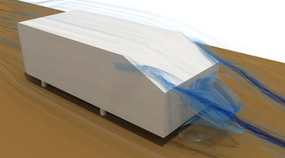
This project will determine the flow behavior by simulating Ahmed's body shape together with a straight road, showing the simulation result plots, and giving the coefficient values obtained in each variation case. Furthermore, the parameters such as velocity and pressure will be shown in contour plots; now, it will be also plotted the acoustical features that are triggered by the pressure gradient around the body.
EQUATIONS
First wall cell height:
`Deltay=(vartheta*y^+)/(u_t)`
where:
`u_t=`Frictional velocity
`vartheta=`Kinematic viscosity
`y^+=`Dimensionless wall distance
Frictional velocity:
`u_t=sqrt(tau_w/rho)`
where:
`tau_w=`Wall shear stress
`rho=`Flow density
Wall shear stress:
`tau_w=1/2c_f*rho*V^2`
where:
`c_f=`friction coefficient
`V=`Free stream velocity
Friction coefficient:
`c_f=0.0576*(Re_d)^(-1/5)`
where:
`Re=`Reynolds number
Dimensionless velocity:
`U^+=V/u_t`
Boundary layer height:
`delta_99=(0.382*L_h)/(Re^(1/5))`
Where:
`L_h=` Characteristic length
growth rate of the wall cells (equation proposed by the author):
`S=(2[(delta_99)/(Deltay)-(n+1)])/(n*(n-1))`
Where:
n= Number of layers
OBJECTIVES
Mesh and refine the meshing generated over the Ahmed body which has been provided by the challenge statements.
Simulate the flow behavior over the geometry meshed, taking into account the road that the body is lying down, is considered as a moving wall.
Determine the main flow features by plotting them in contour plots and convergence plots.
Analyze the sound behavior around the body, by using the "Broadband Noise Sources" tool provided by ANSYS Fluent.
ENGINEERING DEVELOPMENT
- MESHING PROCESS
The geometry provided by the challenge statements is attached below.
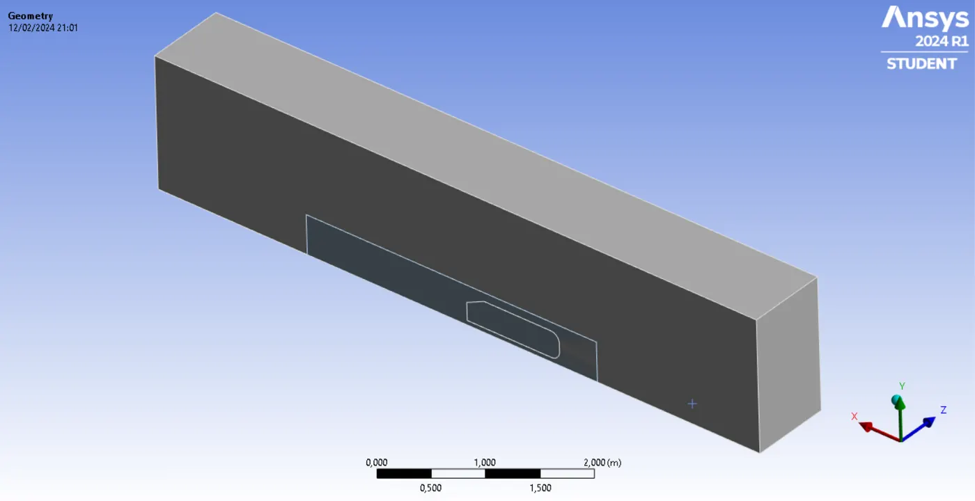
This geometry must be meshed, and the meshing generated over it must be refined. The first step then is to engage the domain body and the density body from the geometry provided, such as the following image shows.
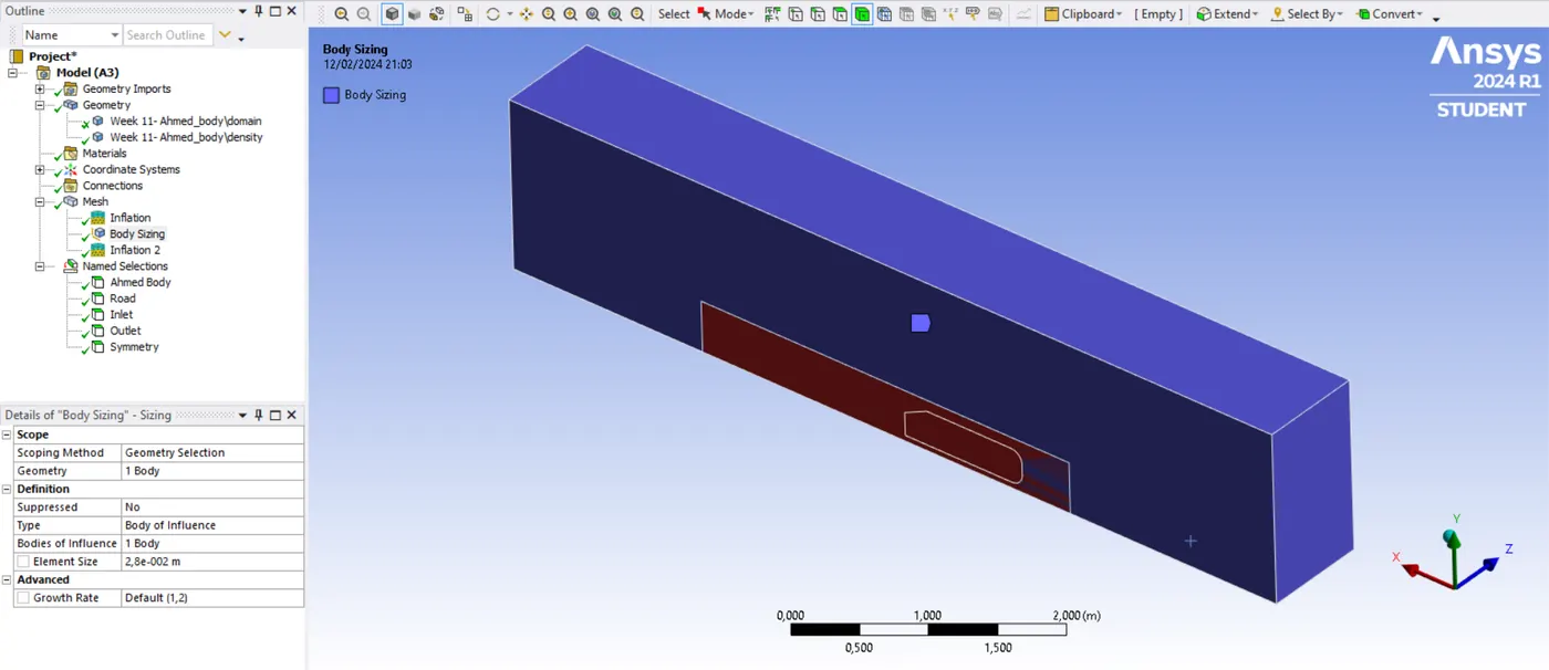
Furthermore, to generate the cells that will consider the turbulence effect over the body surfaces and the road, two inflation tools are generated. However, the body wall cells are calculated by using the equations described above, knowing that the flow is at standard conditions; that means the flow will have the following features:
- Density= `1.225 (Kg)/(m^3)`
- Dynamic viscosity= `1.789*10^-5 (Kg)/(m*s)`
- Kinematic viscosity= `1.48*10^-5 (m^2)/(s)`
The velocity is given by the challenge statements, being approximately:
- Velocity= `31 m/s`
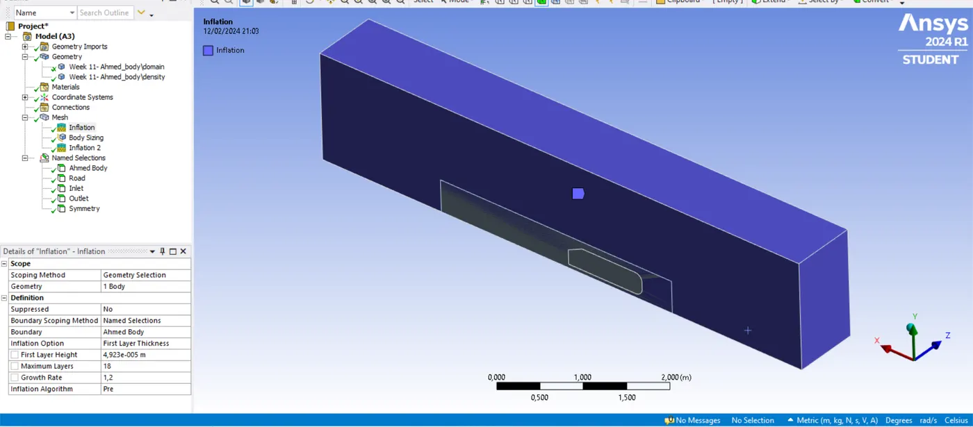
Also, the body has a characteristic length of `1.0989 m`, and its larger cross-sectional area is equal to `0.10408662m^2`. Thus, the results obtained to be entered in the inflation box are:
`Deltay=0.00004923 m`
`delta_99=0.022424m`
`S=1.2`
`n=`18 cells
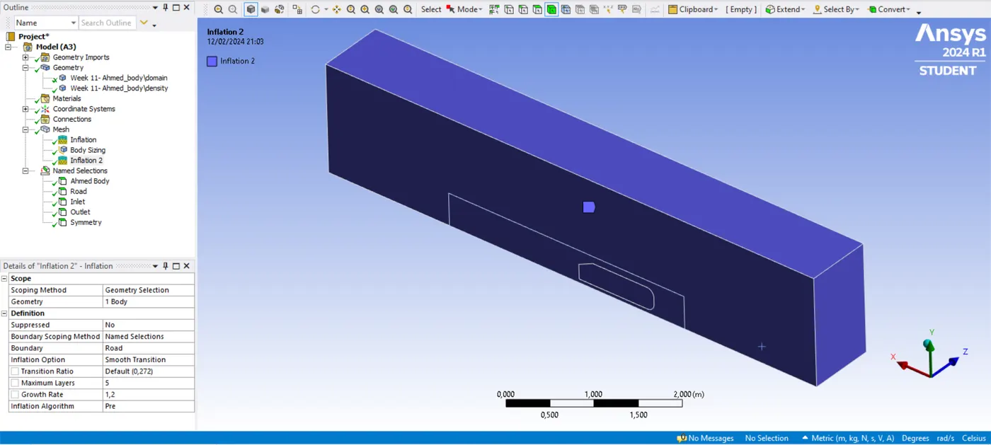
These values are settled in the inflation box as it is shown in the next picture.
The road section just needs to have an aspect ratio of 5.0, with a maximum number of cells of 5, and a growth rate of 1.2.
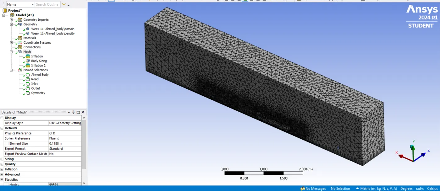
Once the meshing steps described are correctly completed, the body mesh obtained will look like the following picture.
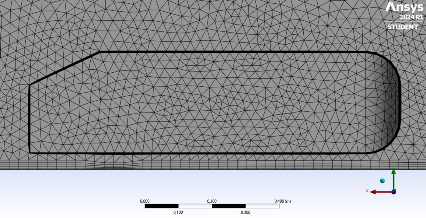
Likewise, the cells that surround the Ahmed's body and the road, must look like a prism cell.
With the meshing process completed, now the simulation process can be performed.
- SIMULATION PROCESS
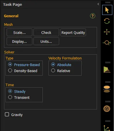
The solver type and other solver features are remained by default.
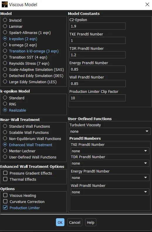
Now, the turbulence model selected is `k-epsilon` Realizable model, with an enhanced wall treatment and a production limiter, to handle the convergence errors. The energy equation is activated together with the turbulence model.
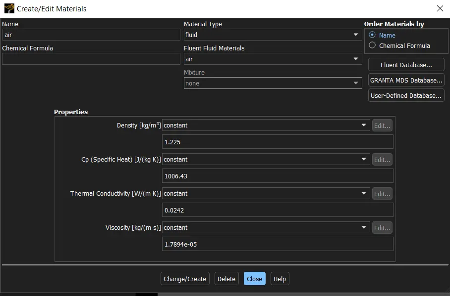
The fluid must have the conditions previously attached, and the density must remain constant because the flow is in incompressible regime.
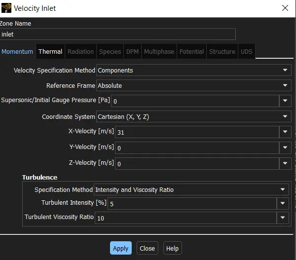
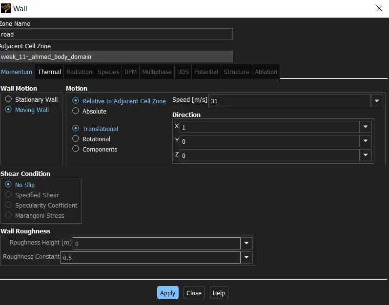
The next step is to enter the velocity described above and activate the moving wall function for the road component.
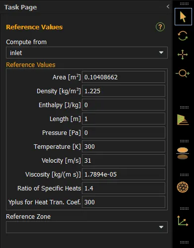
The reference parameters are taken from the inlet, but the reference area must be determined from the cross-sectional area of the Ahmed body, due to the drag and lift coefficient have to be calculated from the flow that passes around the body.
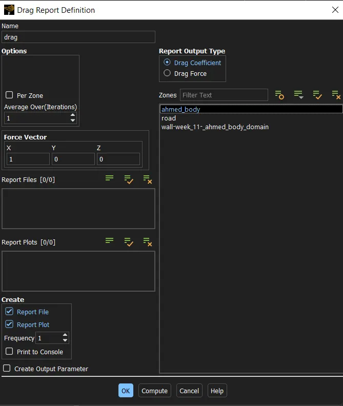
The drag and lift coefficients are plotted using the reports tool.
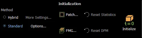
Furthermore, the initialization is performed by using the standard method and selecting the inlet part as the initialization reference.
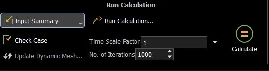
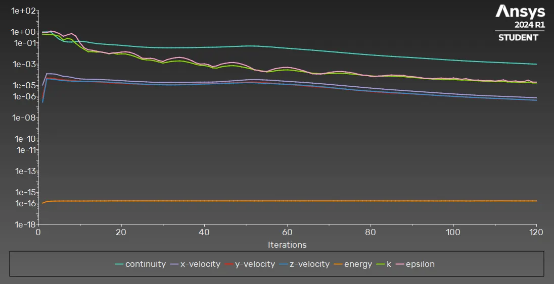
Finally, to run the simulation, the number of iterations taken is 1000, in order to give a great range to find the convergence of the simulation. The simulation will stop once all the solving parameters have obtained an error value of less than 0.001.
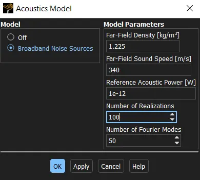
Before or after the solution is obtained, the acoustic model can be activated; the sound behavior solutions will be added to the contour plots slider box, regardless of whether the acoustics tool was activated in whichever of these moments.
RESULTS
The 2D plots obtained from the simulation are:
- Convergence plot
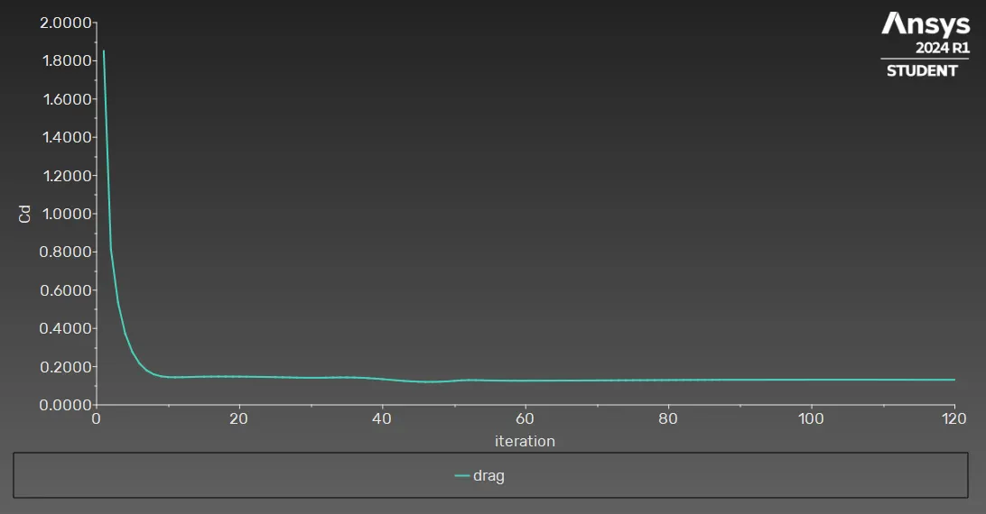
- Drag coefficient
- Lift coefficient
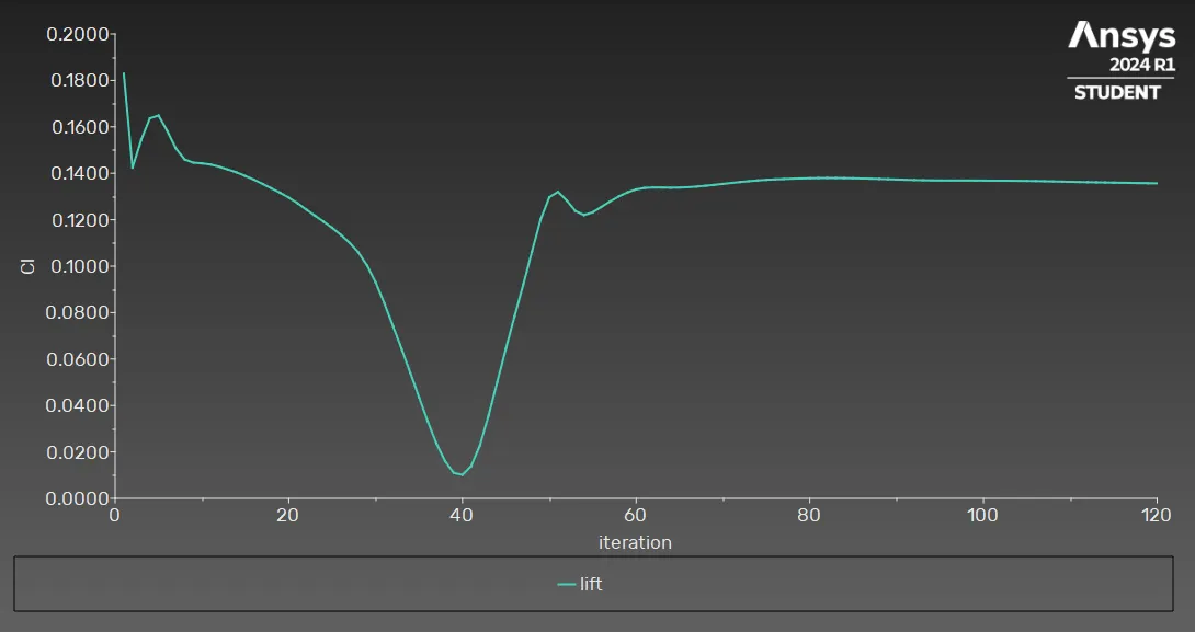
Besides the 2D plots, the lift and drag coefficients obtained are:
| Coefficient | Value obtained (-) |
| Lift coefficient | 0.13566 |
| Drag coefficient | 0.131274 |
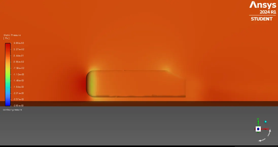
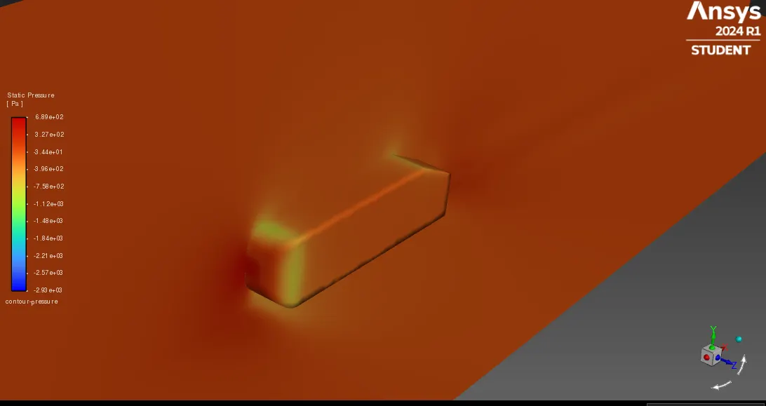
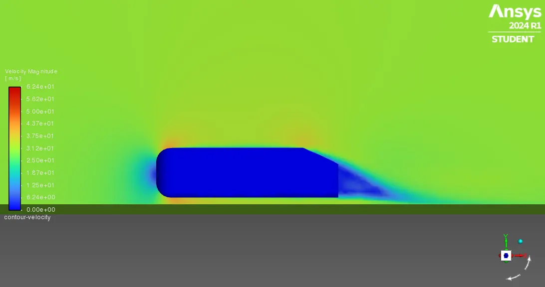
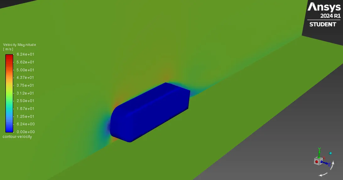
Now, the contour plots of the static pressure, velocity, and acoustic power level in decibels obtained are:
- Static pressure profile
- Front View
- Isometric view
- Velocity profile
- Front View
- Isometric view
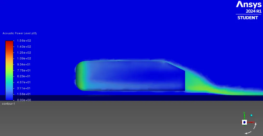
- Acoustic power level (dB)
- Front View
- Isometric view
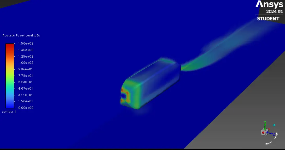
Looking at the results shown above, it can be assumed that the sections where the noise is higher are in front of the body and behind this one; this result is due to the pressure is higher in these two sections than the others. The front section is where the stagnation features predominate, and the behind section is where the flow separation is more noticeable so that the fluid gains more pressure.
CONCLUSIONS
The meshing process could have obtained more accurate results by using a smaller cell configuration if the program had not had the license restrictions; however, the results obtained show good results which can be taken as a reference value for other applications.
The flow separation affects noticeably the flow sound behavior, taking into account that the pressure increases at the sections where the flow is separated, and the sound generated into a flow is caused by the pressure difference.
Broadband noise sources tool can only be used in steady simulations, due to unsteady flow simulations do not obtain accurate results by using this tool; unsteady flows commonly use Ffowcs Williams-Hawkings approximations to solve the sound behavior into a flow field.
REFERENCES