Week 2 - Flow over a Cylinder.
Flow over a cylinder project
AIM
The following project is about the simulation of a flow passing over a cylinder, placed parallel in its longitudinal axis regarding the flow movement. Firstly, the geometry and control volume are drawn on ANSYS software, which is used to simulate different physical behaviors that can occur over some objects, depending on the object working. Once the cylinder geometry and control volume are defined in ANSYS, the next step will be to generate the mesh grid in order to analyze the primitive parameters in different points of the flow which will move into the control volume and over the cylinder. Finally, it will be plotted the lift and drag coefficients in each part of the object body; It must be taken into account the simulation will be performed at different reynolds numbers.
EQUATIONS
Reynolds:
`Re=(VrhoL_c)/mu=(VrhoD)/mu`
Where:
`V=`Velocity
`rho=`Density
`mu=`Dynamic viscosity
`D=`Cylinder diameter
Dynamic viscosity:
`mu=(1.458*10^-6(T)^(3/2))/(T+110.4)`
Where:
T=Temperature
Kinematic viscosity:
`vartheta=mu/rho`
OBJECTIVES
- Establish the initial velocity conditions and the required geometry in order to start the CFD simulation.
- Determine the convergency values for each simulation.
- Plot different primitive parameters and explain why each result changed once the velocity was varied too.
ENGINEERING DEVELOPMENT
Regarding the challenge parameters, there are not specific air parameters, due to that, it will be taken the parameters taken from Bogota, Colombia, where the altitude is approximately 2560 meters:
Air temperature: `T=17°C`
Air pressure: `P=75.6 KPa`
Air density: `rho=0.91 (Kg)/m^3`
Dynamic viscosity: `mu=1.799*10^-5 Pa*s`
Kinematic viscosity: `vartheta=1.977*10^-5 m^2/s`
Even though there are no parameters in the challenge, Challenge statements provides certain Reynolds numbers that will serve for defining velocity values in order to iterate on ANSYS fluent; The reynolds numbers are 10, 100, 1000, 10000 and 100000. Solving the reynolds number equation, the velocity values will be:
`V_(Re=10)=9.885*10^-5 m/s`
`V_(Re=100)=9.885*10^-4 m/s`
`V_(Re=1000)=9.885*10^-3 m/s`
`V_(Re=10000)=0.09885 m/s`
`V_(Re=100000)=0.9885 m/s`
The geometry induced into the flow will be a cylinder with a diameter length of 2 meters and the control volume will be defined as the following way:
- Cylinder diameter
- Volume control length
- Volume control height
Now, the mesh over the surface created above must be refined depending on the surface features and the characteristic zones where the fluid must be clearly analyzed; To do this refinement, it is necessary to use different mesh methods in ANSYS Fluent in order to organize the height and the shape of each element. The mesh methods are:
- Edge sizing:
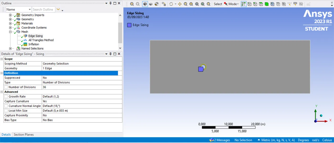
Edge sizing is a mesh tool provided by ANSYS which allows to define the element size around a selected edge. In this case the edge shown in the image simulates the cylinder body and due to that, it must be necessary to take into account the boundary layer over the cylinder in order to obtain more accurate values of different parameters around this shape. The element size will be quadrilateral dominant with a characteristic curve that is generated by the edge shape.
- Method:
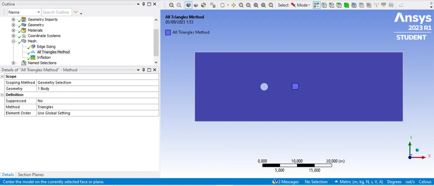
Method is other tool whose main function is to define the type of element shape which will be implemented to analyze each parameter into the volume control. There are three kind of shapes which are:
- Quadrilateral dominant
- Triangles
- Multizone (Quadrilateral and tringles)
In this analysis will be used elements with triangle shapes (unstructured mesh) to see how the fluid behaves in different points passing over the cylinder.
- Inflation:
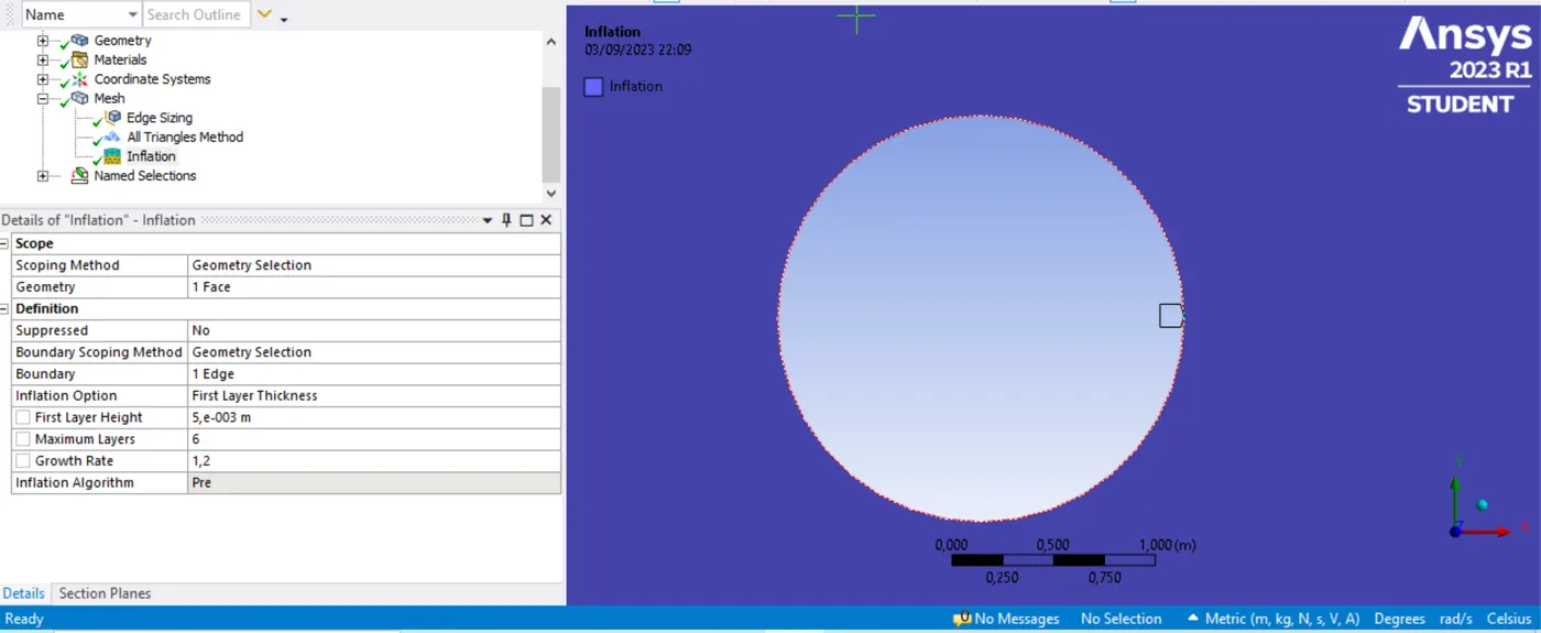
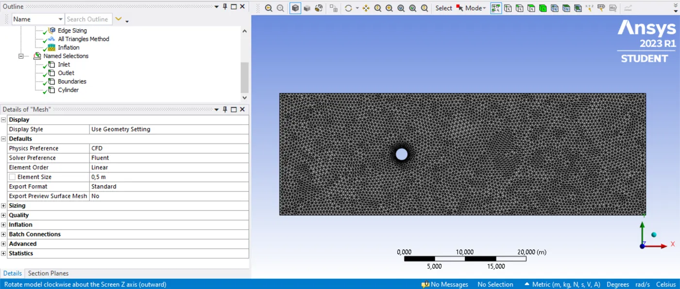
The last method in this simulation is the inflation, which takes the elements applied in the edge sizing method and increases them next to each element. To understand this method is necessary to watch the next picture:
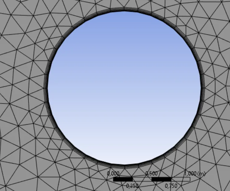
It can be seen around the cylinder, the mesh is a quadrilateral dominant configuration and also, this mesh is increased six times from the cylinder edge. In the image can also be seen the external mesh is divided in triangles as in the second method.
Defined the mesh, it must be carried out the flow simulation. Firstly, the known parameters are entered and the body parts defined as a space stuff. Body parts are divided at:
- Cylinder: Circular object into the mesh
- Inlet: Left side wall
- Outlet: Right side wall
- Boundaries: Top and bottom wall, these ones must be defined as a simmetry on the ANSYS simulation.
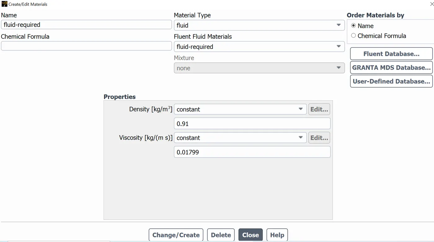
The initial parameters to simulate the flow in steady and unsteady condition are the velocity previously calculated for Re=100. Material used will be Bogota air density, then, the parameter is pudated into the material icon as it is shown in the following image. Viscosity changing is explained below, once the velocity increasing is explained too.
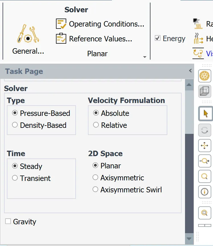
To vary the type of solver, it can be found clicking on general icon and then, searching the solver function. It is shown in the image below:
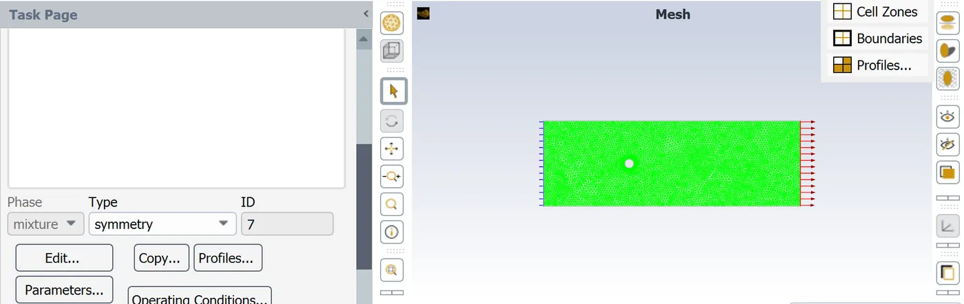
Once the solver and the wall-fuction solver (laminar for this particular case) are chosen, the next step is to define the space function that each body part will accomplish. Boundaries will play as a infinite part of the space; to assign this function, it is required to use the function "simmetry" implemented on type of boundaries in boundary icon.
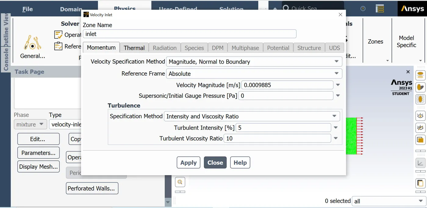
Inlet will content different velocities depending on the reynolds number which wants to be analyzed, however, in the image is shown the velocity obtained above for Re=100, this velocity is too low due to the length of the cylinder diameter and, furthermore, the low viscosity that the fluid has. To get an accurate result, the values at 100 Reynolds will be multiplied by 1000, so the velocity will be 0.9885 and viscosity will be 0.01799 Kg/(m s); this method will be used in all the velocity values in order to get the most real values that the simulation should obtain.
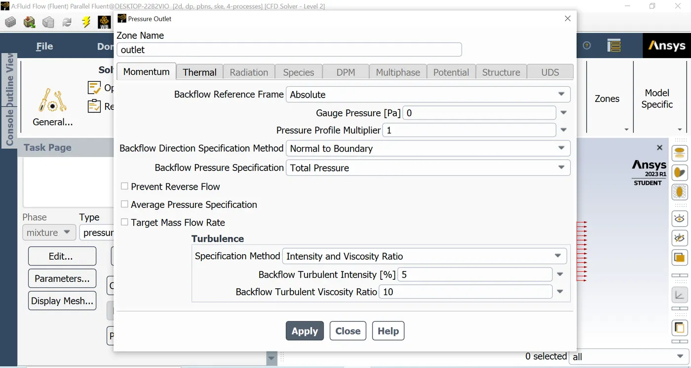
Outlet will just content the pressure at the outlet of the control volume, which wil firstly be 0 Pa, in order to the program recalculate this one.
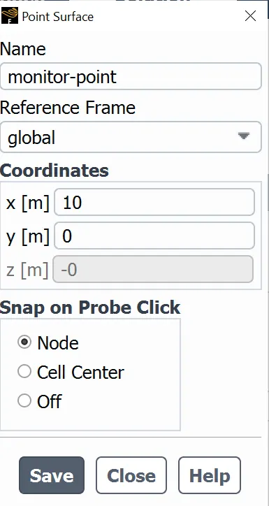
It is also added a point that serves for analyzing the velocity in a determining spot of the volume control. This is called monitor point and it is located according to the following image:
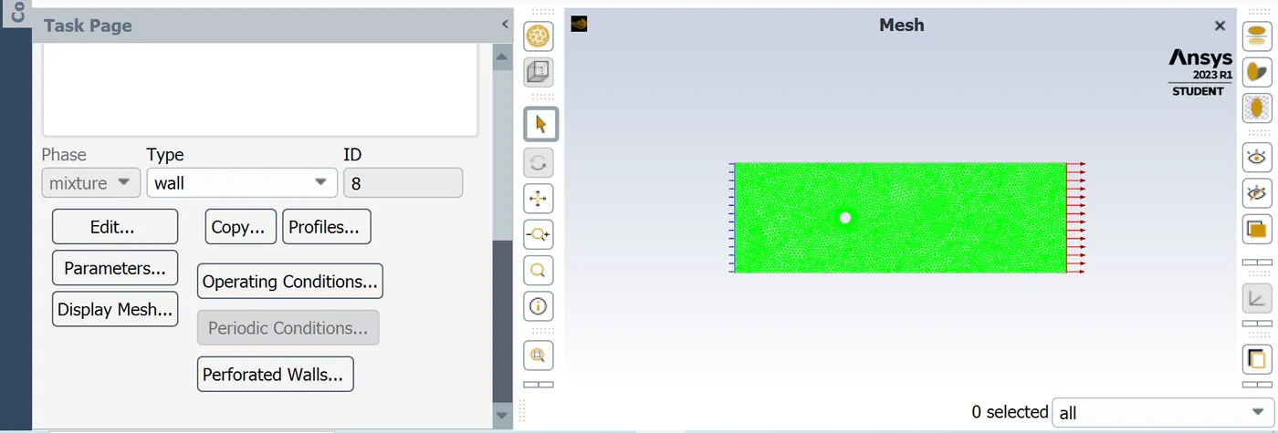
Cylinder is taken as a wall and finally, the inner cylinder section is not considered.
Once the body part parameters have been defined, it is now necessary to generate the reports that are required. The reports are:
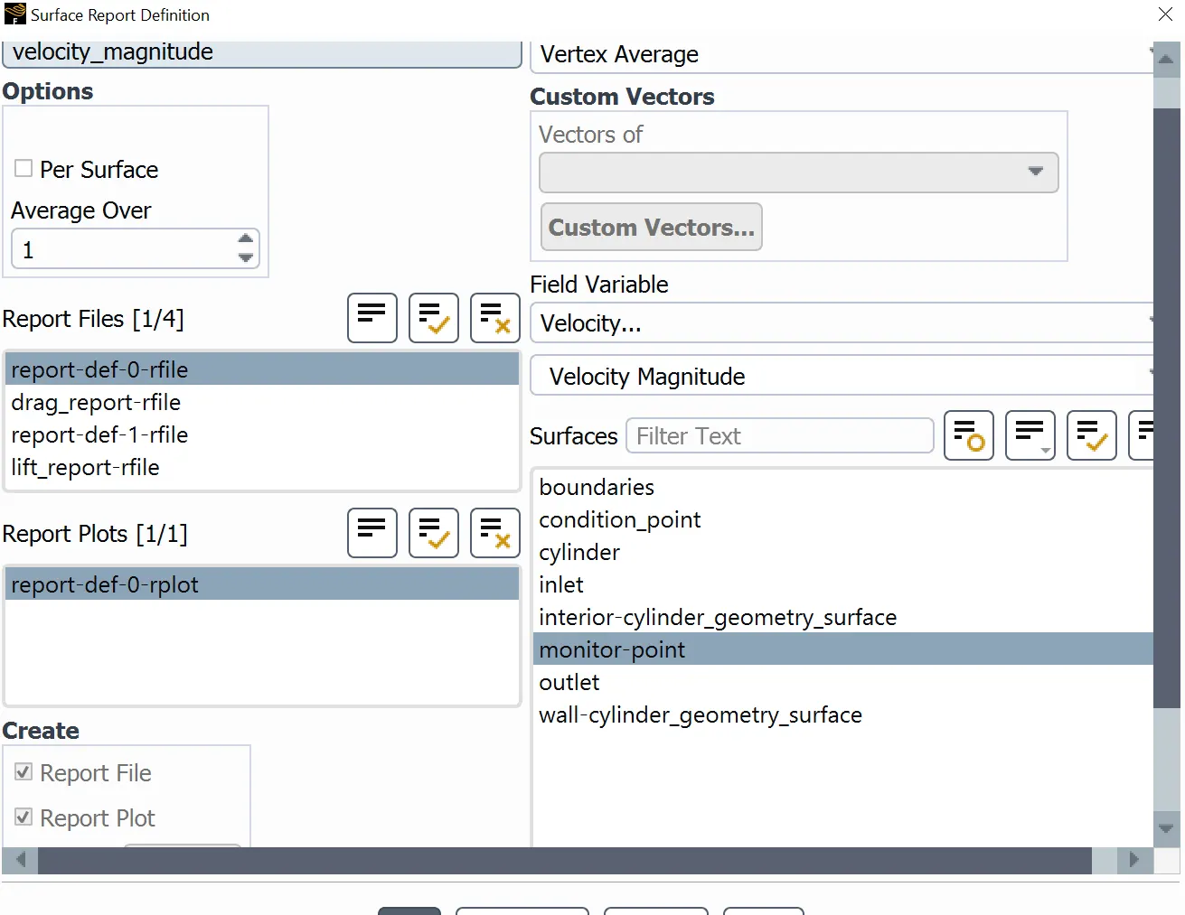
- Velocity magnitud at the monitor point
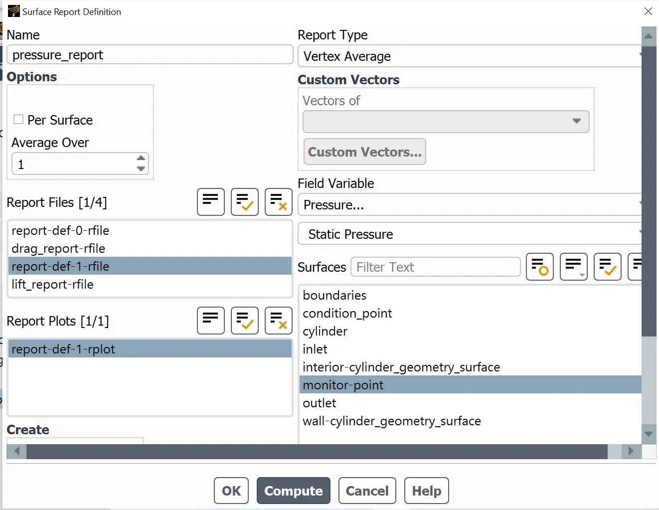
- Static pressure at the monitor point
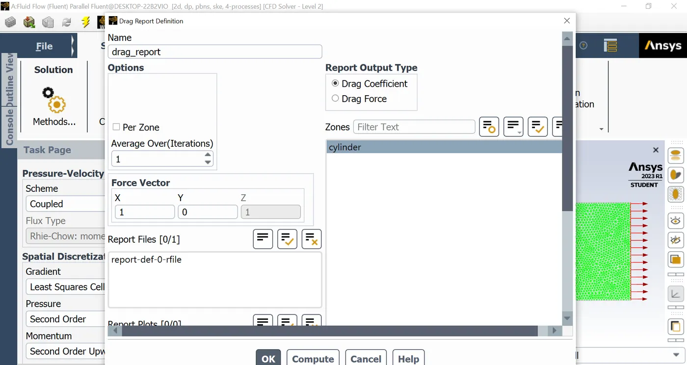
- Drag coefficient
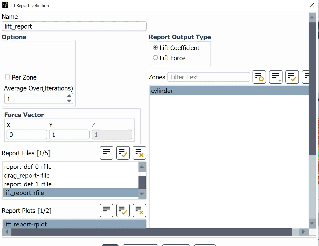
- Lift coefficient
- Strouhal number (flow fluctuation rate): Strouhal number is an well-known value in CFD due to this value represents the oscillation of the flow unstability when this one is perturbed by an object moving into the flow. A general calculation of the average Strouhal number can be calculated as the following way:
`St=(omega*L)/V`
Where:
`omega=`oscillation frequency
`V=` flow velocity
`L=` characteristic length
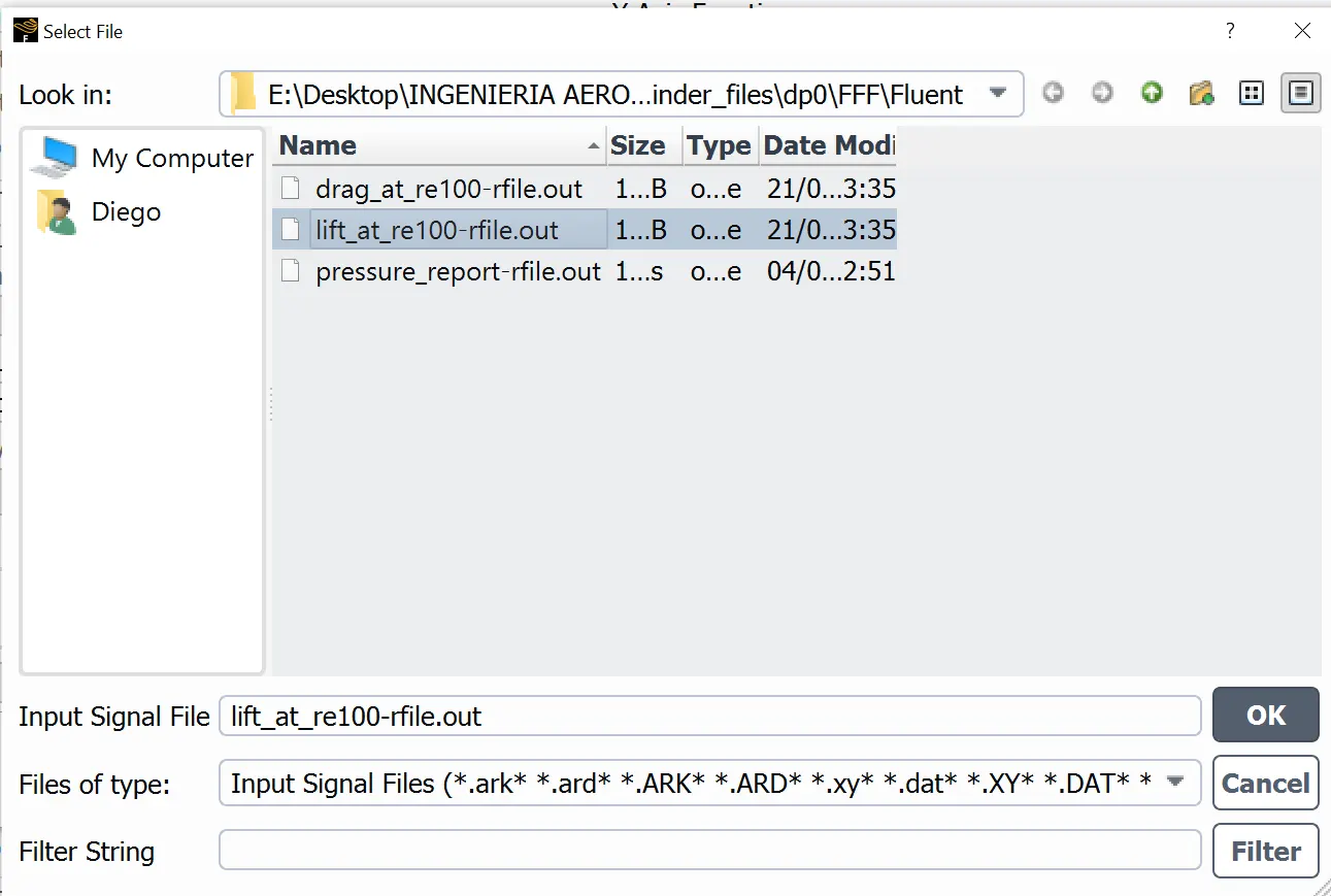
To get Strouhal number will be firstly necessary to obtain the maximum value of lift coefficient, however, because of the lift coefficient won't be linear, otherwise the fluid will have some perturbations, it must be used the function FFT provided by ANSYS, in order to arrange the lift results obtained in the cases where the convergency is like a wave function. For running the simulation, it will be taken some iteration values as in steady as in transient solver.
Then, once the solution has been plotted, FFT function is used:
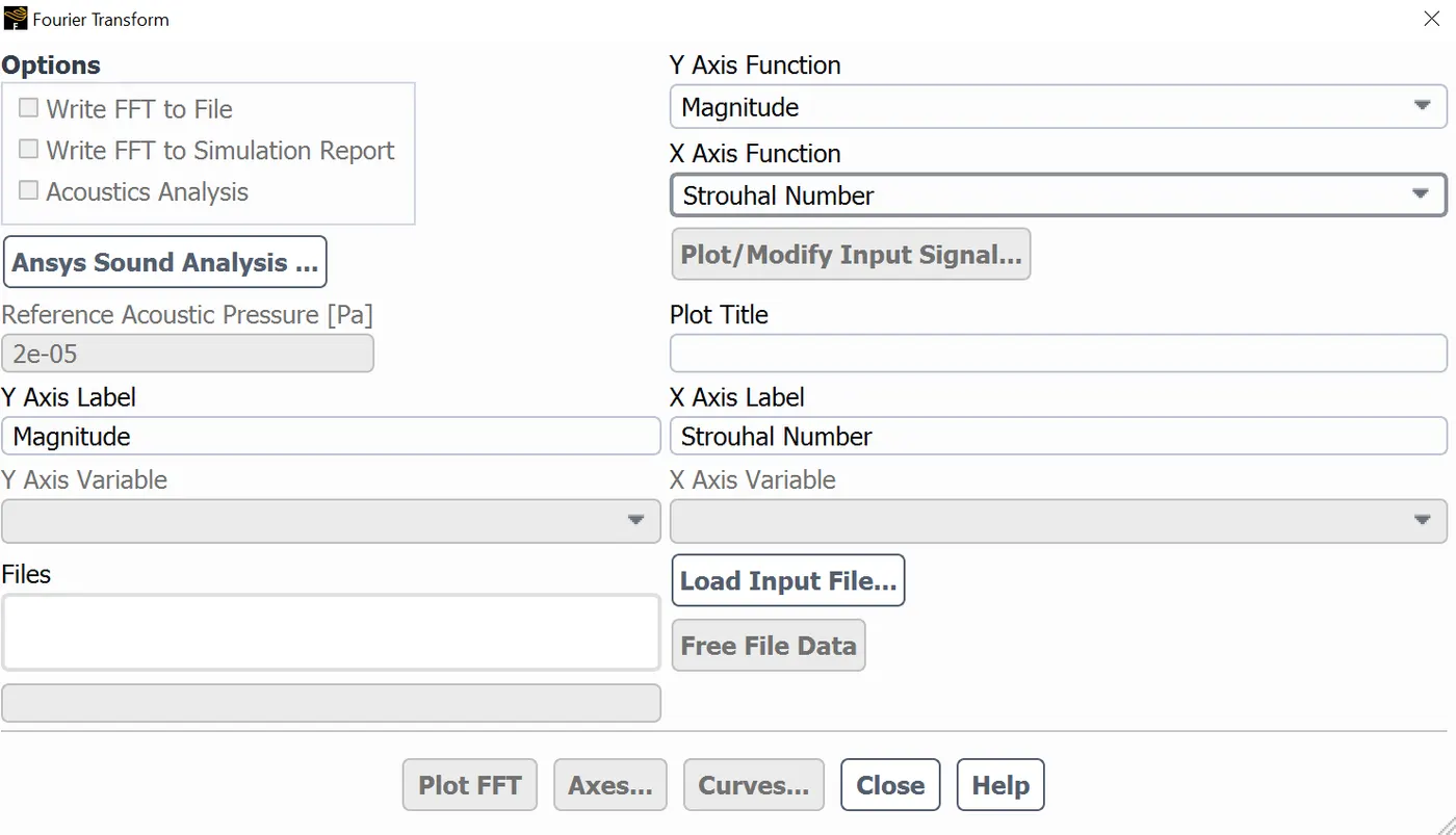
All the values rearranged by FFT are entered in an excel and, with some excel loops, the strouhal number is obtained.
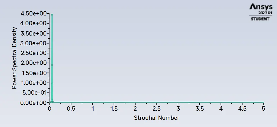
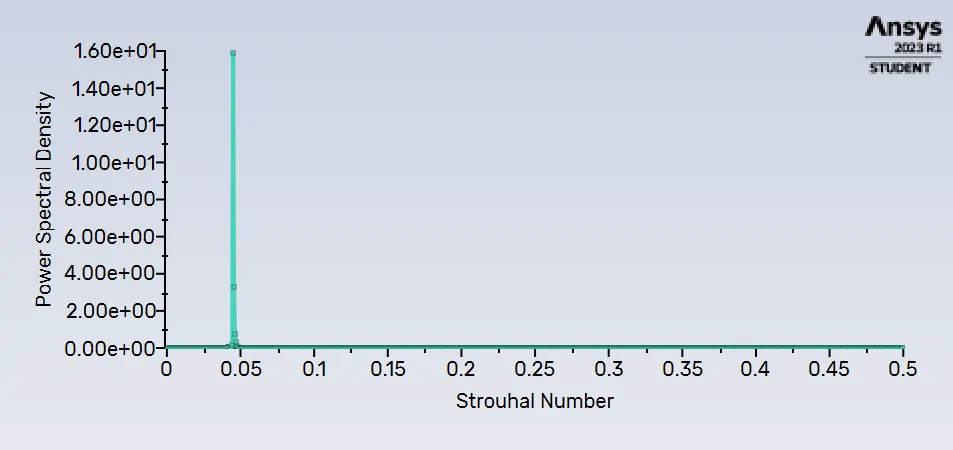
Selecting the "Plot FFT" button, ANSYS will show the following graph, where the strouhal numer is the maximum peak of the graph.
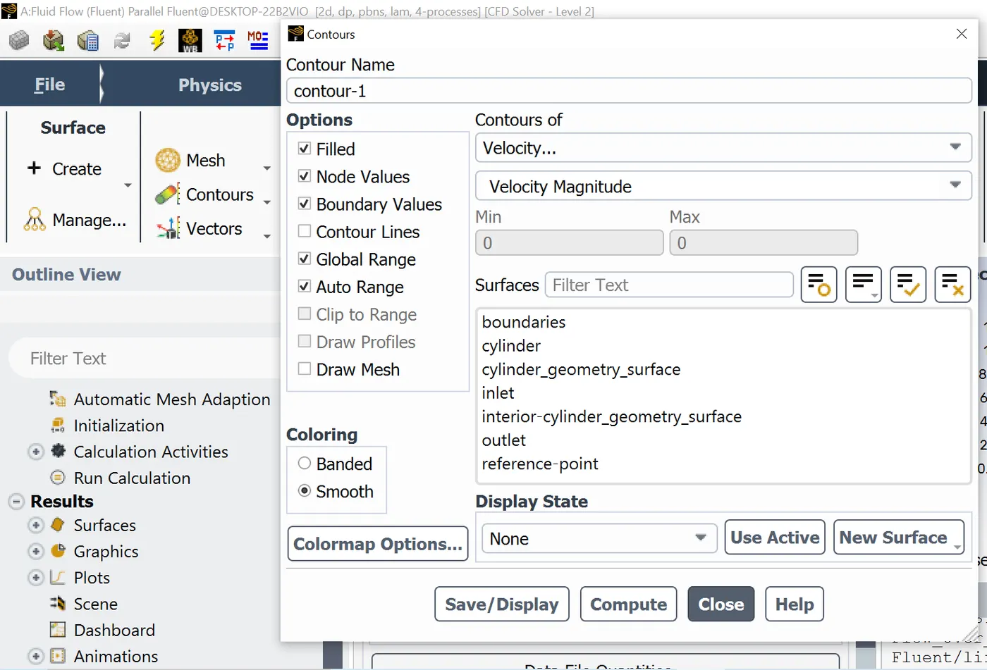
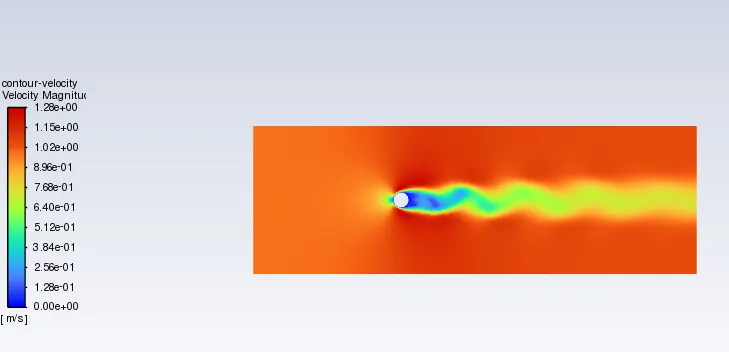
Engineering development process explained is repeated to the other simulations required. Also, to watch the flow behavior around the cylinder and inside the control volume, it is used the "contour" function, located at "Results" icon.
RESULTS
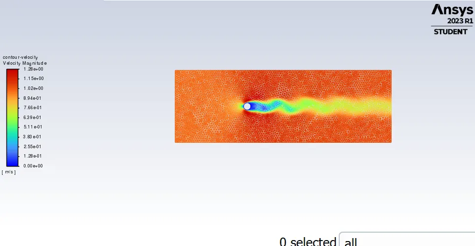
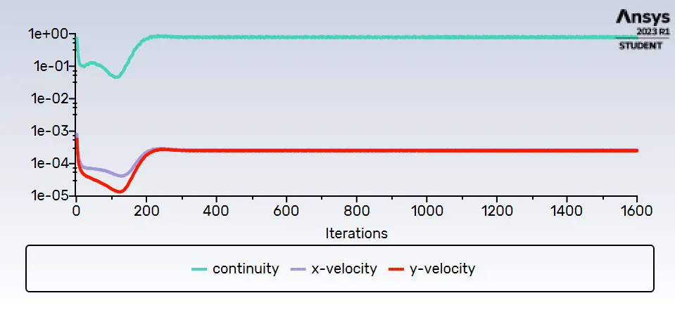
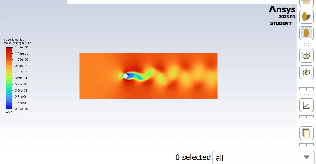
The flow in all the cases began to gain perturbations which did not get easier to get a certain convergency; however, lift, drag, velocity and pressure always kept the similar wave behavior as is shown in the following images:
- Flow behavior at steady case for Re=100
Strouhal number plot:
- Convergency:
- Flow behavior at unsteady case for Re=100
Strouhal number plot:
- Convergency:
| Parameter | Steady | Transient |
| Lift coefficient | 0.1502 | 0.3335 |
| Drag coefficient | 1.31 | 1.4 |
| Strouhal number | 0.0463 | 0.0681 |
Karman Vortex Shedding and its relation with Strouhal number
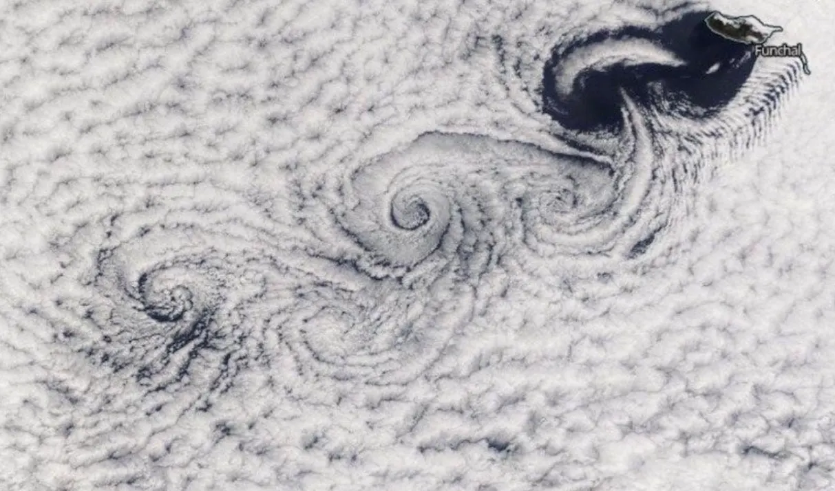
Karman vortex is known in fluid mechanics as the fluid frequency triggered by the flow shedding. All newtonian and non-newtonian fluids will be perturbed on its stream lines once the fluid particles have touched any solid object or fluid with different velocity, pressure and/or temperature; Karman vortex phenomena occurs when fluid particles,with a determined velocity, close to any object are touching the object walls, they will begin to lose kinematic energy due to the friction against the object wall and then, the stream lines near from this particles affected, will be affected too, triggering a flow messy over the object; Karman vortex phenomena looks like:
Reviewing the Strouhal number equation, it can be noticed there is a parameter which represents the fluid oscillation frequency, in ohter words, this is the Karman value, and it can be calculated by taking the lift coefficient frequency obtained in the simulations. Therefore, in the two simulations performed above (Steady and transient for Reynolds 100), flow oscillation is obtained, but it is more clearly in transient simulation, because of the transient function takes the time as a convergency factor and also, in each step-time, the program is looking for getting an accurate value in this determined step-time. To get certain of the results obtained, these ones are compared with simulations performed by other people; the results obtained by different investigations are:
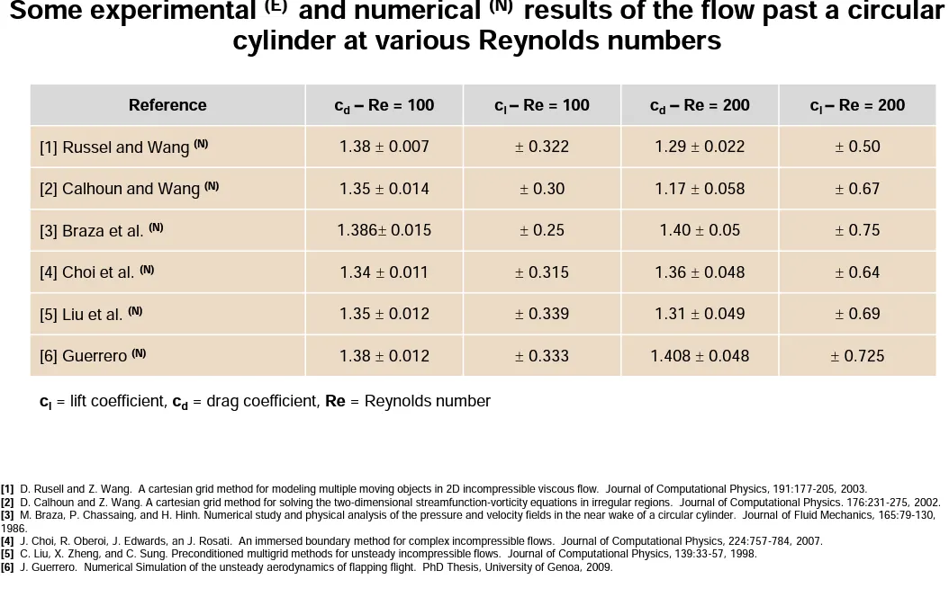
Image taken from: http://www.wolfdynamics.com/wiki/tut_2D_cylinder.pdf
So, carrying out a mean value between those results and the results obtained in this project for transient, the eror will be:
| Description | Lift Coefficient | Drag Coefficient |
| Mean Value Calculated | 0.3098 | 1.36433 |
| Project Value Obtained | 0.3335 | 1.4 |
| % Error | 2.37 | 3.57 |
It is already determined the simulation is acomplishing with the standard results that are normally obtained under the conditions used into this project.
Lift and Drag Coefficients at different Reynold numbers
Velocity values of each Reynolds number are shown above at the beggining of this project, however, in some cases due to the ANSYS Fluent parameters takes wrong Lift and Drag values, perturbing the ideal results, it will only be varied the viscosity value once the reynolds number is equal or greater than 1000. The results obtained in each simulation are:
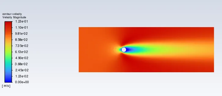
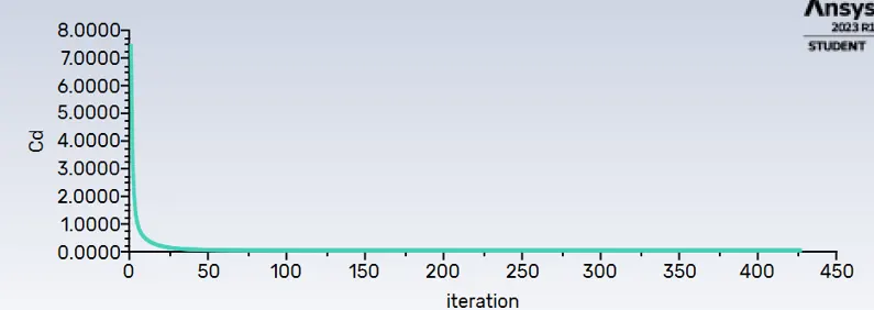
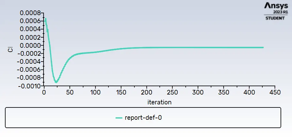
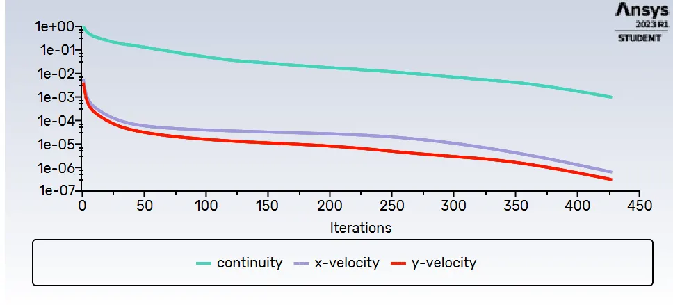
- Reynolds = 10 ;Flow velocity=0.09885 `m/s`; Dynamic viscosity = 0.01799 `(Kg)/(m*s)`(Air viscosity incread x1000); Density = 0.91`(Kg)/(m^3)`
Drag:
Lift:
Convergency:
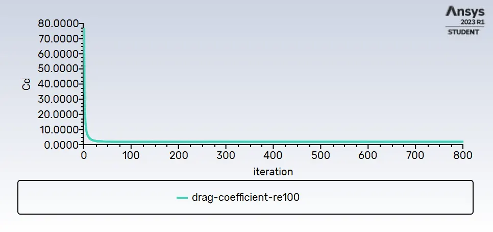
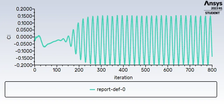
- Reynolds = 100 ;Flow velocity=0.9885 `m/s`; Dynamic viscosity = 0.01799 `(Kg)/(m*s)`(Air viscosity incrased x1000); Density = 0.91`(Kg)/(m^3)`
Drag:
Lift:
Convergency:
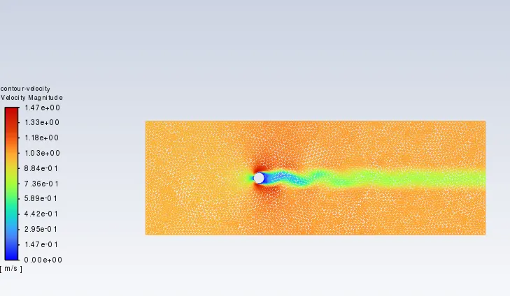
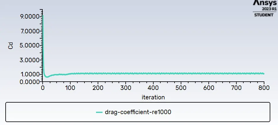
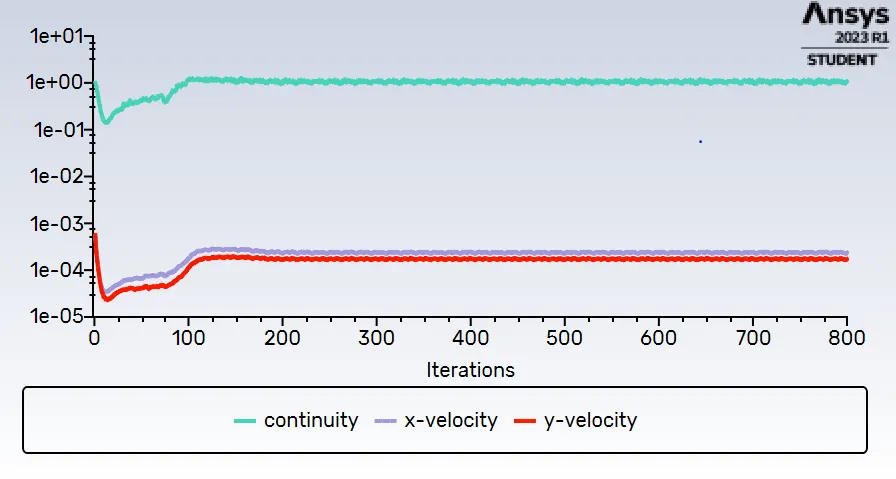
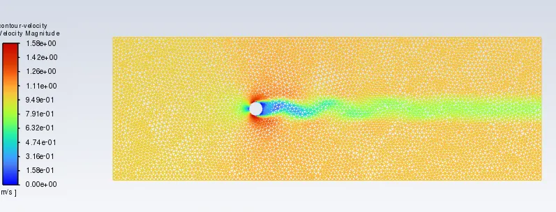
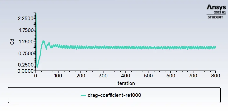
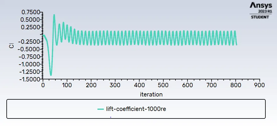
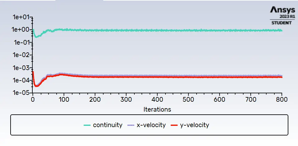
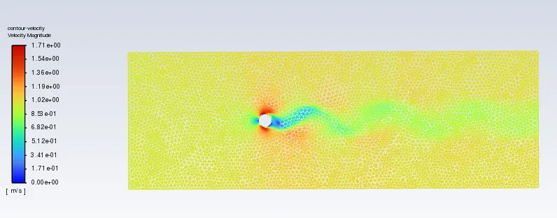
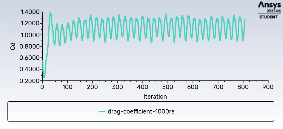
- Reynolds = 1000 ;Flow velocity=0.9885 `m/s`; Dynamic viscosity = 0.001799 `(Kg)/(m*s)`(Air viscosity increased x100); Density = 0.91`(Kg)/(m^3)`
Drag:
Lift:
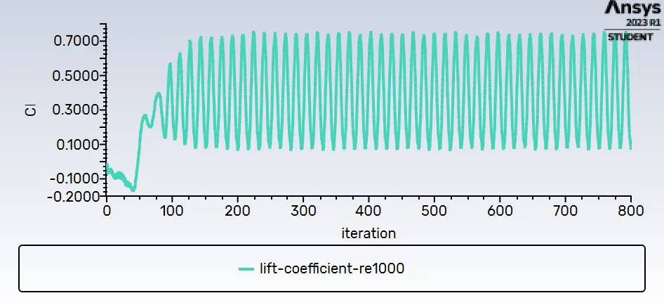
Convergency:
- Reynolds = 10000;Flow velocity=0.9885 `m/s`; Dynamic viscosity = 0.0001799 `(Kg)/(m*s)`(Air viscosity increased x10); Density = 0.91`(Kg)/(m^3)`
Drag:
Lift:
Convergency:
Reynolds = 100000;Flow velocity=0.9885 `m/s`; Dynamic viscosity = 0.00001799 `(Kg)/(m*s)` (Air viscosity without increasing); Density = 0.91`(Kg)/(m^3)`
Drag:
Lift:
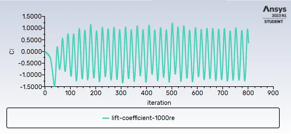
Convergency:
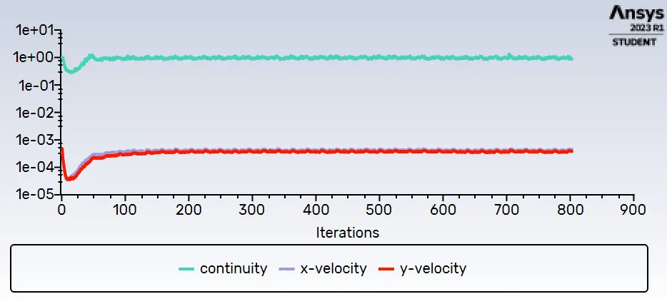
NOTE: The simulation was performed on the same project, due to that in some descriptions 1000re is shown; do not take into account this issue.
General results:
| Reynolds number | Lift Coefficient | Drag Coefficient |
| 10 | 0.000123 | 0.0478 |
| 100 (Steady) | 0.1502 | 1.31 |
| 100 (Transient) | 0.3335 | 1.4 |
| 1000 | 0.43 | 1.12 |
| 10000 | 0.254 | 0.974 |
| 100000 | 0.144 | 1.127 |
CONCLUSIONS
Regarding the results obtained in steady and transient simulations for reynolds 100, it is clearly deducted the best way to simulate the flow behavior over a cylinder should be by transient function; this function will always take the most accurate strouhal number value, because of the simulation also takes step-time to carry out a solution. Furthermore, due to the low that the Reynolds number is, the program is always going to calculate the lift and drag coefficient values taking just into account the velocity provided, so these coefficient values may not be the certain values in comparison with the values that should be obtained. It is adviced to vary the velocity and the reference values (viscosity) if it is necessary.
In the second section, Reynolds 10 is a clearly example of laminar flow without any perturbation, due to that, it is not possible to get an strouhal number. The laminar flow without perturbation is kept until the Reynolds number is greater than 50.
Reynolds at 100 and 1000 value show the vortex shedding behind the cylinder, because of the flow velocity is enough high that the simulation achieves the flow perturbation.
At Reynolds 10000 and 100000 are also obtained the flow shedding but, the drag and lift coefficient , especially drag coefficient, reach an inconsistent perturbation where the coefficient values get local and global peaks, but in order to get the same result that should be obtained in the previous simulations, it must be carried out a simulation using turbulence methods, taking into account the flow becomes turbulence once the Reynolds value is greater than 4000.
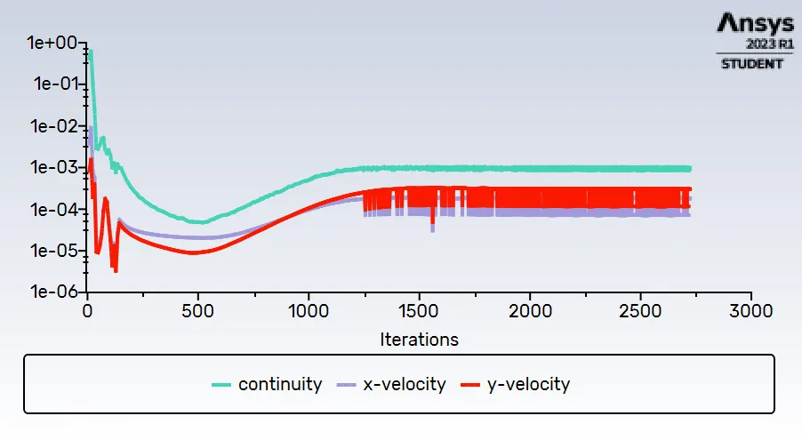
Convergency is assumed once the convergency plot reaches a linear oscillation where the error percentage is increases and decreases just an a maximum and minimum constant value; this assumption just apply for simulations where the flow does not remain stable. In the very low Reynolds case Re=10, it is easily to determine the solution have converged.
That's it, thank you for reading.
REFERENCES
https://www.engineeringtoolbox.com/international-standard-atmosphere-d_985.html
https://www.omnicalculator.com/physics/kinematic-viscosity-of-air
https://www.engineeringtoolbox.com/strouhal-number-d_582.html