Week 5 - Rayleigh Taylor Instability
Rayleigh Taylor Instability
AIM
The following project will be developed in order to watch and analyze the behavior between two combined fluids closed into a control volume and disturbed by the gravity force. This fluid phenomena es well-known as Rayleigh-Taylor Instability and it occurs when a heavy fluid is dropped into a ligth fluid, these two fluids will seek a way to dwon the potential energy gained by the gravity force and particle smashes, until they both reach a stability. However, due to the energy exchange, the two fluids lose their initial properties, making the fluid density is varied at different heigth points.
To perform the Rayleigh Taylor Instability analysis will be used air and water, putting the water fluid up to the air fluid in its initial condition. It will be firstly developed the geometry zone where the fluids will be contented; then, it will be carried out mesh refinement, using three different mesh sizes and after that, it will be simulated the fluid behaviors regarding the time change. Finally, it will be plotted the behavior by means of videos which show the fluid behavior in each time step.
It is also important to take into account a number known as Atwood number, which is used in hydrodynamics to determine the instability in density-stratified flows. It will be forward analyzed what happens with the fluid behavior once the Atwood number is varied.
EQUATIONS
- Atwood number:
`A=(rho_1-rho_2)/(rho_1+rho_2)`
Where:
`rho_1=`Fluid density of the heavy fluid
`rho_2=`Fluid density of the light fluid
OBJECTIVES
Model the control volume where the two fluids will interact each other and their respective meshes.
Simulate the Rayleigh Taylor instability in different mesh size and density cases, using transient functions to solve each simulation.
Determine the flow behavior and the dynamic movement between the particles regarding the time change, until the fluids reach a potential energy stabilization.
Analyze the behavior variation due to the density variation and explain the importance of Atwood number in this fluid phenomena.
ENGINEERING DEVELOPMENT
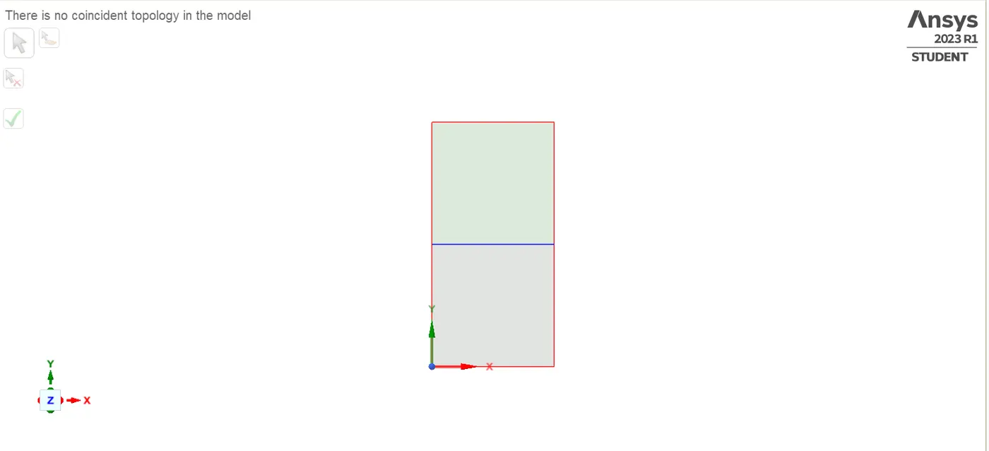
The main geometry zone which will content the two fluids, is shown below. There will be two squares, one over the other one, and those two will represent the air fluid (bottom square), and the water fluid (top square). Using "share" tool allows the mesh between the squares is always aligned; the blue line at the middle of the two squares will get certain the share tool was correctly applied.
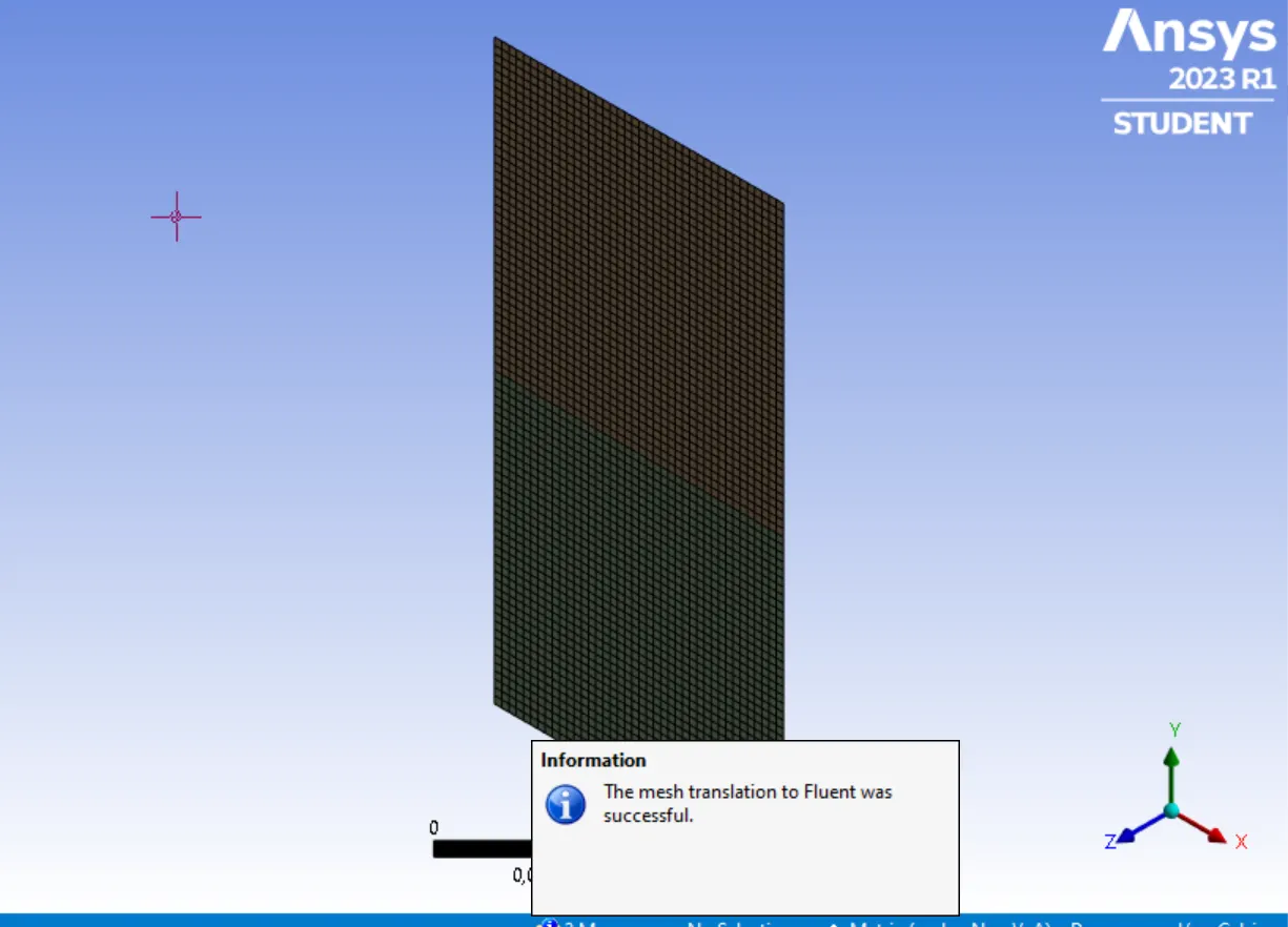
Once the geometry has been created, the next step is to generate the geometry mesh and refine it. In this case is not too complex to refine the mesh, because of the geometry does not have complex shapes. The mesh on the geometry is shown in the following picture.
It will be used three different mesh sizes, such that the simulation will be approximated to an accurate solution. The three cases has the following features:
| Cases | Elements | Nodes |
Element size (m) |
Water density (`(Kg)/(m^3)`) |
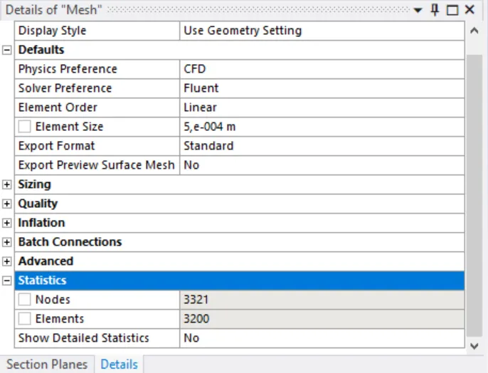
| I | 3200 | 3321 | 0.0005 | 988.2 |
| II | 80000 | 80601 | 0.0001 | 988.2 |
| III | 12800 | 13041 | 0.00025 | 400 |
Features shown above are obtained by reviewing the table provided by the ANSYS mesh tools, at the left-side from the bottom. The icon called "details of Mesh" looks like the image below.
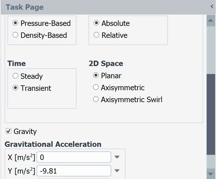
Now, with the mesh created, it can be carried out the flow simulation. Firstly, the type of function solver, and the Time solver are entered and also, the gravity is used in this analysis, due to the one of the main factors that the phenomena is triggered by the potential energy that the heavy fluid gains once this is released and starts dropping, being combined with the light fluid. The gravity acceleration value is equal to 9.81 downwards the y axis.
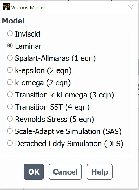
Likewise, the predominant model which the correct simulation is reached, is using laminar flow, due to the initial velocity of every fluid is equal to zero and, there is not any single object that can disturbe anyone fluid, triggering turbulent flows.
Furthermore, to achieve a realistic behavior model which the two fluids will get, it is also necessary to use a mathematical model known as Multiphase. Multiphase is, as it was written, a mathematical model that describes the physical behavior of two materials which have been combined, but they have different states of phase or chemical properties. Multiphase has four solver models, depending on the primitive parameters that the fluids have as initial condition. The models are shown in Multiphase Model icon from ANSYS Fluent.
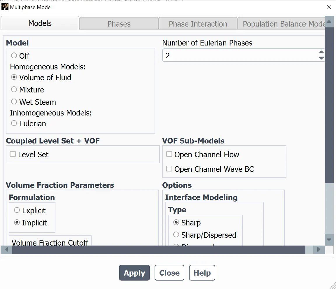
ach model is mainly used for:
1. Volume of Fluid: It is commonly used for tracking the volume fraction into each cell from the mesh domain, taking into account three main physical equations. These equations are:
- Volume fraction equation
- Momentum equation
- Energy equation
This method only works in Pressure-based method.
2. Mixture Model: Mixture model is used when each fluid immerse into the domain has different velocities and it is commonly used in liquid-solid flows. The equations involved in this model are:
- Volume fraction equation
- Momentum equation
- Continuity equation
- Energy equation
This model works efficiently using pressure-based method.
3. Wet Stream Model: The model is a combination of Eulerian approach and the mixture model, but the fluid features cannot be varied due to the equation is already fixed with the standard conditions that the fluids have in normal conditions. This model is only used fot density-based method and uses the same equation models that are used on Mixture model.
4. Eulerian Model: This model can calculate the volume fraction along the domain, combining multiple phases like solid, liquid and gas all together; however, this is limited by the convergency and it is also assumed the all phases have only single pressure. The equations used for solving this model are:
- Volume fraction equation
- Momentum equation
- Continuity equation
- Energy equation
To get more information about the multiphase model and all the equations, do not doubt to enter in the following link: https://lms.skill-lync.com/programs/94933/23/multiphase/knowledgebase
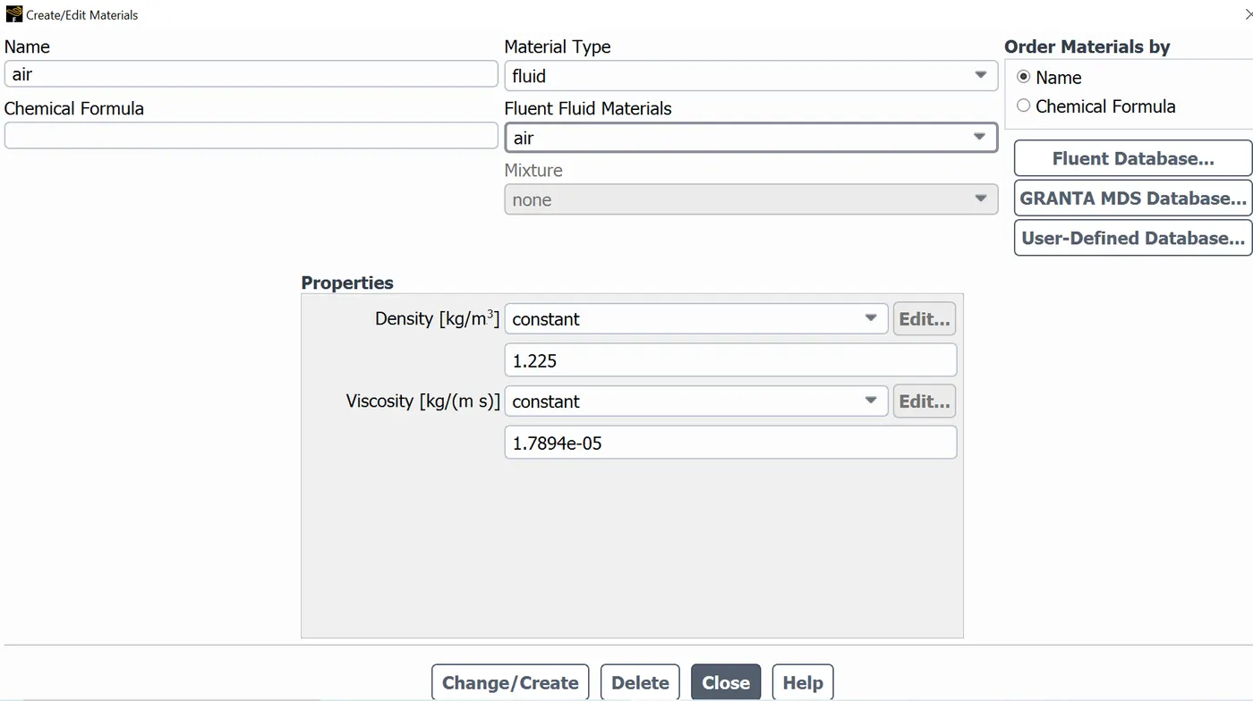
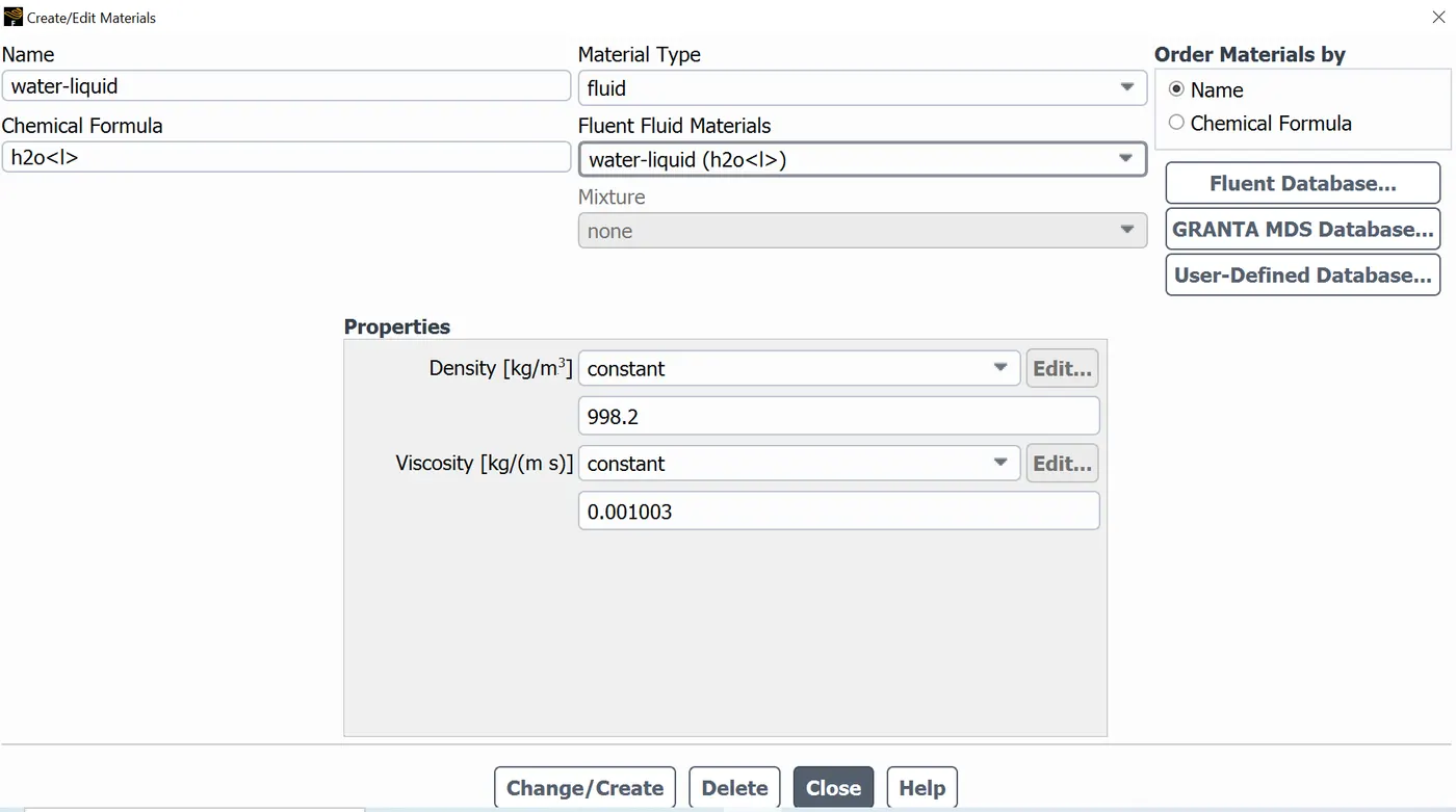
There are another Multiphase models that are not provided by ANSYS, but in this particular case, it is used Volume of Fluid method, because of this model is better to simulate the volume fraction behavior, varying the particle pressure magnitude as it should be in a real experiment. Besides selecting the solver methods and the solution model, it is also defined the fluids used in this simulation, which are air and water; the water density will be varied as is shown in the third picture below, in order to watch the flow behavior with different fluid features.
- Air features:
- Water features (Case I & II):
- Water features (Case III):
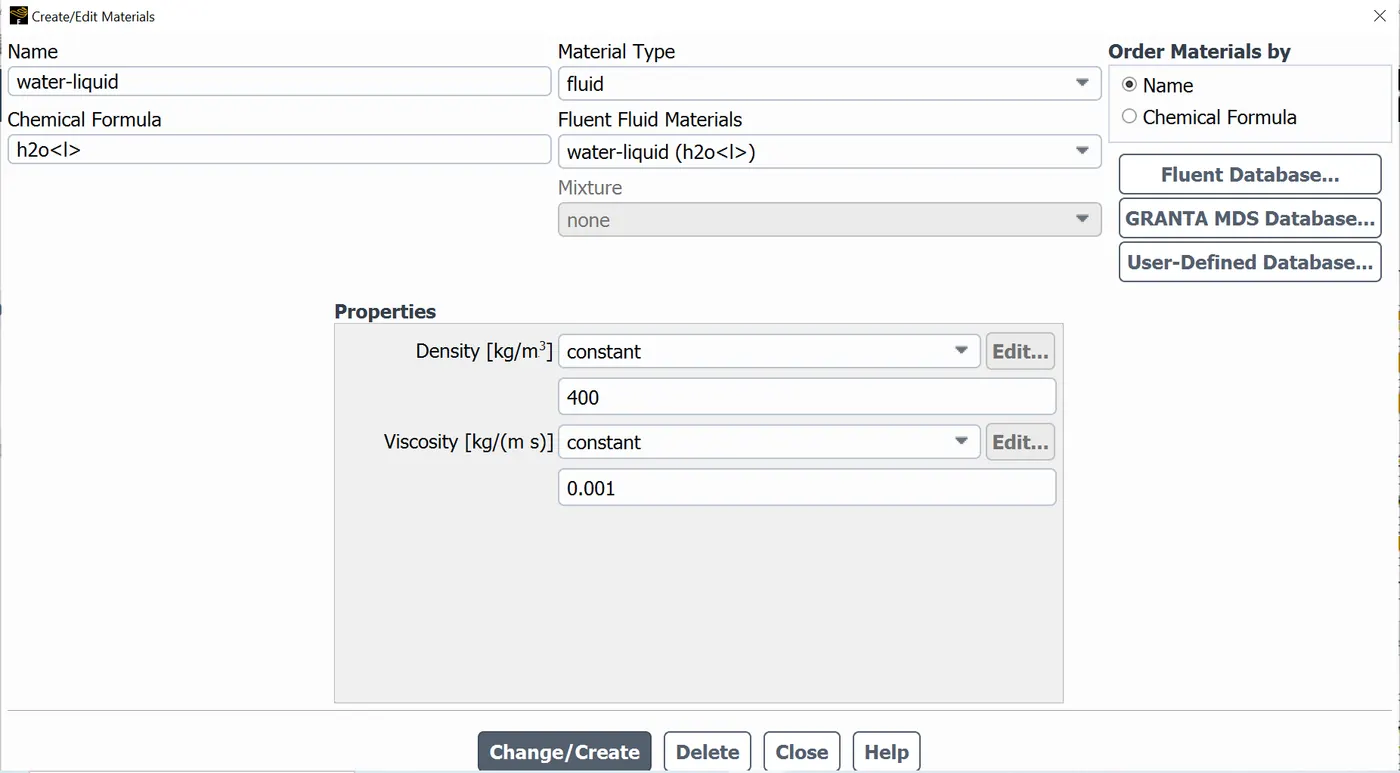
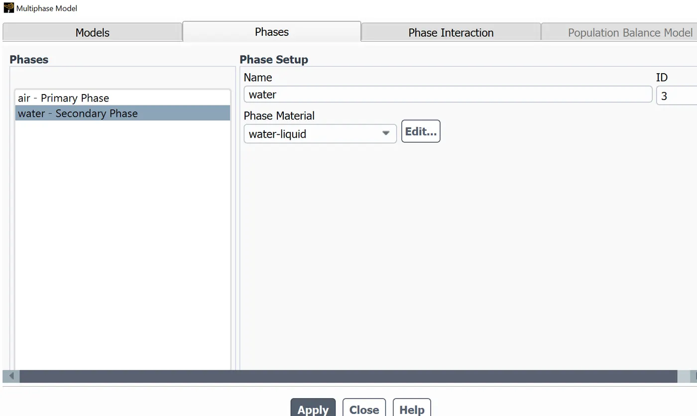
At the same way, into the Multiphase model icon are defined what fluid will be each one.
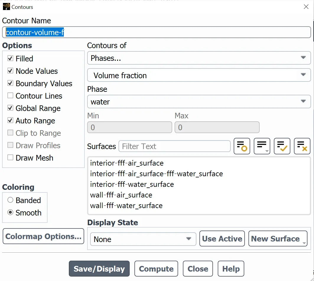
To watch the fluid movement in each step, it is created a contour plot which will serve for generating a plot animation that will save each iteration result that will get the simulation in every time step.
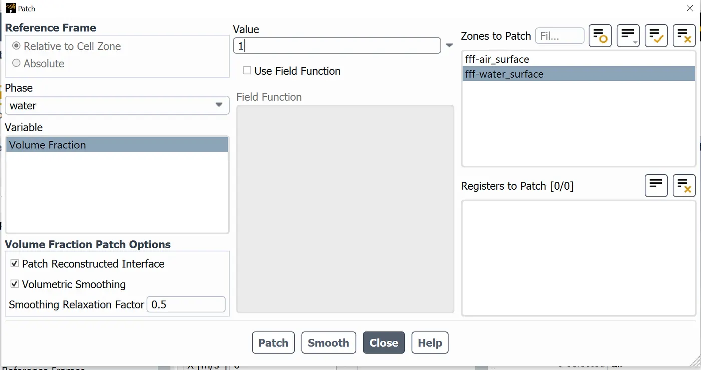
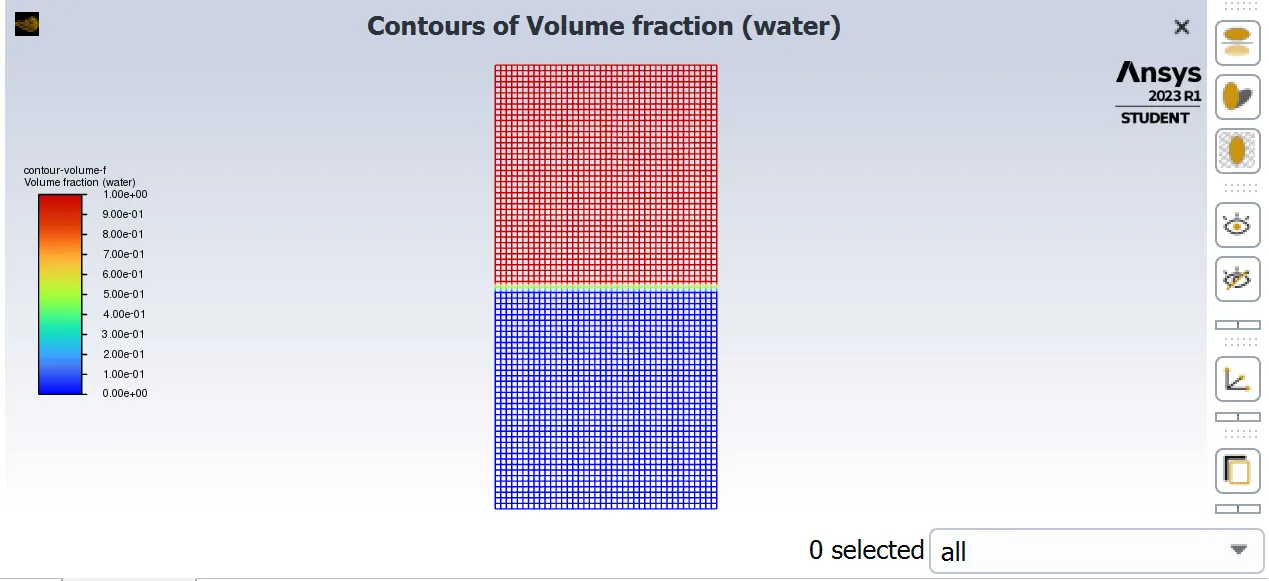
It is then used the patch function, due to the inicialization will not get anything if the geometry surfaces are not named into the simulation. In this case, the predominant volume fraction is the water and the mesh will show the volume fraction as a percentage value which will be 1 if the mesh cell has only water inside or 0 if the mesh cell has only air instead. To get certain the patch function was correctly entered, the initial contour plot must be plotted as it is shown in the second picture below.
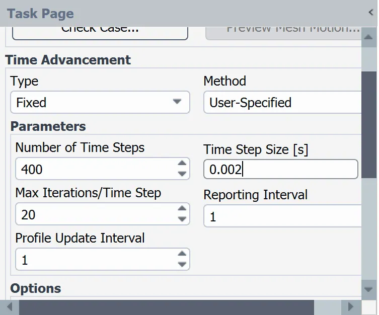
Finally, to run the calculation, the CFL number has to be carefully taken; so, the time-step selected can not be greater than a CLF number equal or less than 0.5.
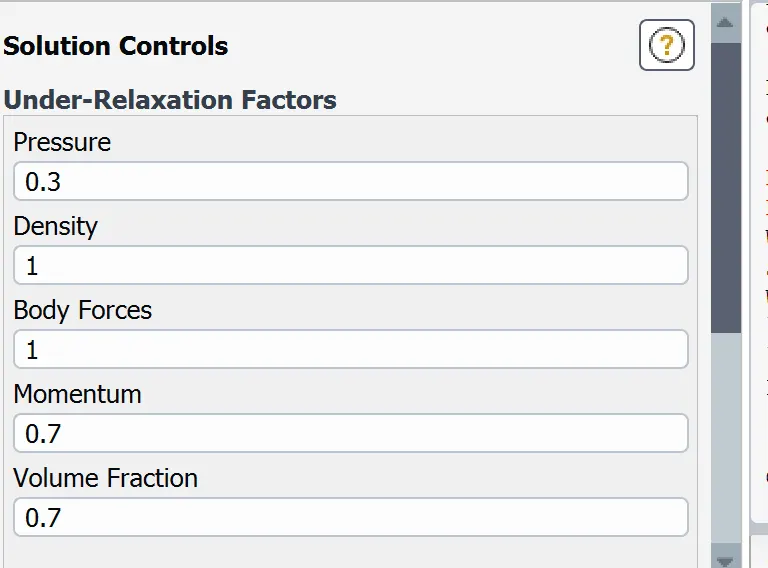
At lower mesh sizes occurs an issue known as FPE (Floating-point exception), that is found out if the program finds a aritmethical operation that can not be solved or in other words, the program has found a divergence. To get rid of this problem, it may be necessary in much cases to vary the Under-relaxation factors, using the pressure and velocity values as 0.3 and 0.7 respectively. This trouble was obtained in the second case and it was overcame using the Under-Relaxation configuration shown in the following picture.
RESULTS
The results obtained in each case are:
Case I (Iterations taken = 700; Time-steps = 0.005):
Link: https://youtu.be/vSTFKm-gEoQ
Atwood number= 0.998
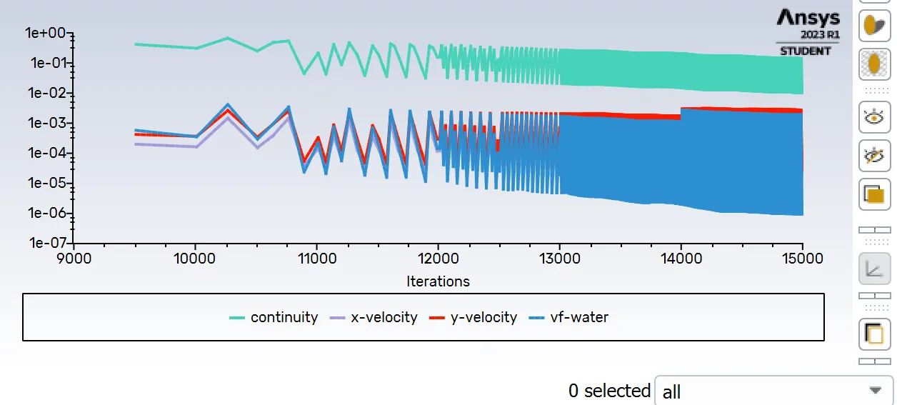
Case II (Iterations taken = 1500; Time-steps = 0.002):
Link: https://www.youtube.com/watch?v=lRyWwSZdDSE
Atwood number= 0.998
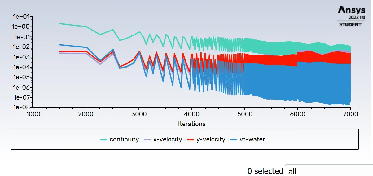
Case III (Iterations taken = 700; Time-steps = 0.005):
Link: https://www.youtube.com/watch?v=ZgP8r1ZAOWk
Atwood number= 0.994
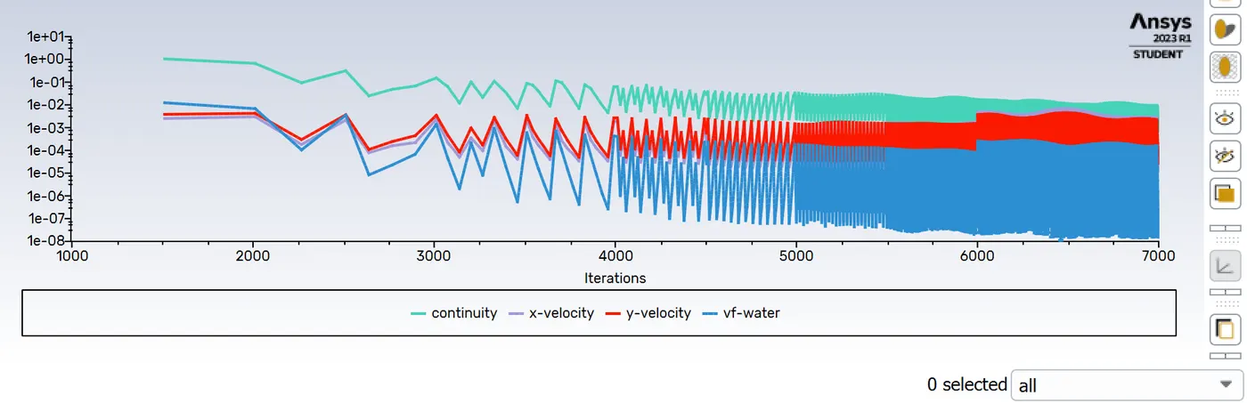
It is initially determined the solution convergency at the second case will take more iterations due to the time sloop is shorter than the first and third case. This delay is due to even the time-steps had been reduced, the solution diverged and the under-relaxation variation helped solving the simulation. Furthermore, comparing the first two cases results with the third one, it is clearly determined the colour contour is not alike in all the cases , because of the third case contour plot varies its colour divisions, getting a less concentration of water at the bottom section, due to the density decreasing.
CONCLUSIONS
The Awood number shows the density of the fluid will have an important weigth into the fluids combination, showing the fluid volume fraction was weaker once the fluid density was decreased. Likewise, the fluid stabilization is faster in a fluid with greater density, because of the fluid weigth gets the fluid particles combined split up quicker than a fluid lighter.
The simulation is not suitable using Steady-state function, due to the fluid will not be the same every time and steady-state will only seek the fluid convergency in a single time-step. Similar cases of instability where the flow behavior is not always constant, must be carried out using transient-state functions.
Rayleigh-Taylor instability has different ways to be solved, however, each fluid has different conditions and due to that, the behavior can vary from one model solver to other model solver. To get certain the fluid combination is correct, it is necessary to use an appropiate solution model by reading the main function of each of these models.
REFERENCES
http://www.scholarpedia.org/article/Rayleigh-Taylor_instability_and_mixing
https://www.sciencedirect.com/science/article/abs/pii/037015739190153D
https://academic-accelerator.com/encyclopedia/atwood-number
https://lms.skill-lync.com/programs/94933/23/multiphase/knowledgebase