Week 4.1 - Genetic Algorithm

Genetic algorith function code and three sutdy cases:

%Genetic Algorithm
%Diego Alejandro Cepeda Cuartas
clear all
clc

%Firtsly we're going to start creating a mesh 
x=linspace(0,0.8,150)
y=linspace(0,0.8,150)

[xx,yy]=meshgrid(x,y)

%Then, we have to evaluate the stalagmite function for obtaining the plot
for i=1:length(x)
    for j=1:length(y)
        vec(1)=xx(i,j);
        vec(2)=yy(i,j);
        sf(i,j)=ga_function(vec);
    end
end

%Plot the function 
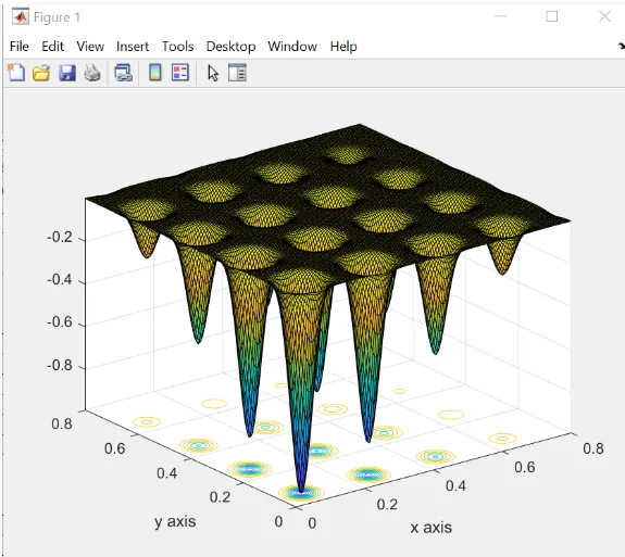
surfc(x,y,sf)
xlabel('x axis')
ylabel('y axis')

%Generating the genetic algorith for the fitness function analysis 
[input,fval]=ga(@ga_function,2)


% Now, we are going to stimate the Global Maxima in three different kind of
% studies: 

% Study 1-Statistical behavior without iterations 

%Number of iterations
number_cases=50

%genetic algorith calling 
tic
for i=1:number_cases
    [inputs,foptim(i)]=ga(@ga_function,2);
    xoptim(i)=inputs(1);
    yoptim(i)=inputs(2);
end
study1_times=toc

%Statistical behavior plot 
figure(1)
subplot(2,1,1)
xlabel('x axis')
ylabel('y axis')
hold on
surfc(x, y, sf)
shading interp 
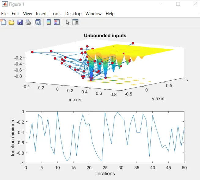
plot3(xoptim,yoptim,foptim,'marker','o','markersize',5,'markerfacecolor','r')
title('Unbounded inputs')
subplot(2,1,2)
plot(foptim);
xlabel('iterations')
ylabel('function minimum')

%Study 2-Statistical behavior with upper and lower boundaries 

%genetic algorithm calling 
tic
for i=1:number_cases
    [inputs,foptim(i)]=ga(@ga_function,2,[],[],[],[],[0:0],[1:1]);
    xoptim(i)=inputs(1);
    yoptim(i)=inputs(2);
end
study2_time=toc

%Genetic algorithm with boundaries defined plot
figure(2)
subplot(2,1,1)
xlabel('x axis')
ylabel('y axis')
hold on
surfc(x, y, sf)
shading interp 
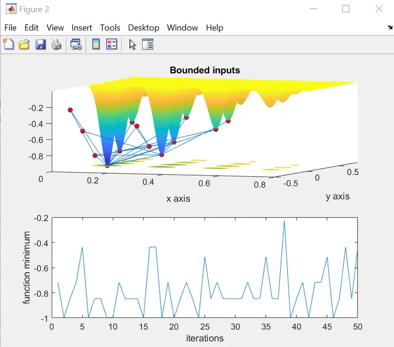
plot3(xoptim,yoptim,foptim,'marker','o','markersize',5,'markerfacecolor','r')
title('Bounded inputs')
subplot(2,1,2)
plot(foptim);
xlabel('iterations')
ylabel('function minimum')

%Study 3-Statistical behavior increasing the iterations values 
%Increasing the size of the population 
increase=optimoptions('ga');
increase=optimoptions(increase,'PopulationSize',600);

%genetic algorithm calling 
tic
for i=1:number_cases
    [inputs,foptim(i)]=ga(@ga_function,2,[],[],[],[],[0:0],[1:1],[],[],increase);
    xoptim(i)=inputs(1);
    yoptim(i)=inputs(2);
end 
study3_time=toc

%Genetic algorithm increasing the iterations number plot
figure(3)
subplot(2,1,1)
xlabel('x axis')
ylabel('y axis')
hold on
surfc(x, y, sf)
shading interp 
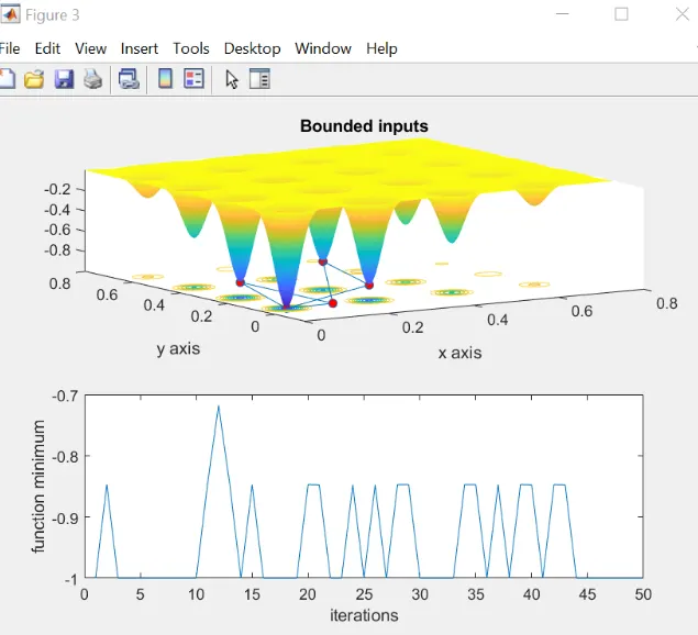
plot3(xoptim,yoptim,foptim,'marker','o','markersize',5,'markerfacecolor','r')
title('Bounded inputs')
subplot(2,1,2)
plot(foptim);
xlabel('iterations')
ylabel('function minimum')

%Global maxima point 
close all
clear all
clc

%creating the mesh
x=linspace(0,0.8,150);
y=linspace(0,0.8,150);
[xx,yy]=meshgrid(x,y);

%for plotting the surface of stalagmite
for i=1:length(xx)
    for j=1:length(yy)
    input_vector(1)=xx(i,j);
    input_vector(2)=yy(i,j);
    f(i,j)=ga_function(input_vector);
    
    end

end
surfc(xx,yy,-f)
shading interp

%evalutaing the function
increase=optimoptions('ga','PlotFcn',{@gaplotbestf,@gaplotstopping},'populationsize',200);
[x,foptim]=ga(@ga_function,2,[],[],[],[],[0;0],[1;1],[],increase)

xoptim=x(1);
yoptim=x(2);

figure(1)
hold on
plot3(xoptim,yoptim,-foptim,'marker','o','markersize',5,'markerfacecolor','r')

Stalagmite function code sheet:

%Stalagmite code 
%Diego Alejandro Cepeda Cuartas


function [GA]=ga_function(in)
x=in(1);
y=in(2);

%Stalagmite function 
f_1x=(sin(5.1*pi*x+0.5)).^6;
f_1y=(sin(5.1*pi*y+0.5)).^6;
f_2x=exp((-4*log(2))*(((x-0.0667).^2)/0.64));
f_2y=exp((-4*log(2))*(((y-0.0667).^2)/0.64));

GA=-(f_1x.*f_1y.*f_2x.*f_2y);% The minus serves for getting the correct value
end 

Genteic Algorithm Document Link:

https://docs.google.com/document/d/1AHUsn492CeYWlAJUX50nSbZuvSGBNjaE_QZ18zMXzcE/edit?usp=sharing

Plots obtained:

- Stalagmite function plot:

- First study case plot result:

- second study case plot result:

- third study case plots results:

- With 200 Iterations:

- With 300 Iterations:

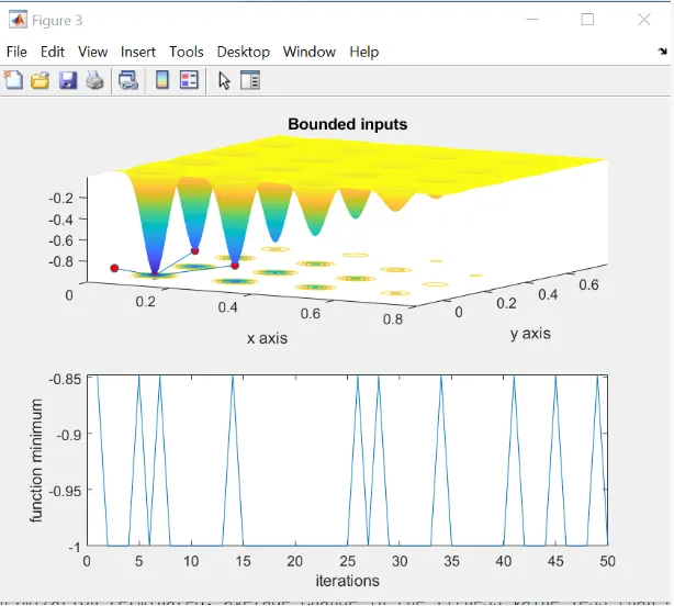
- With 350 Iterations:

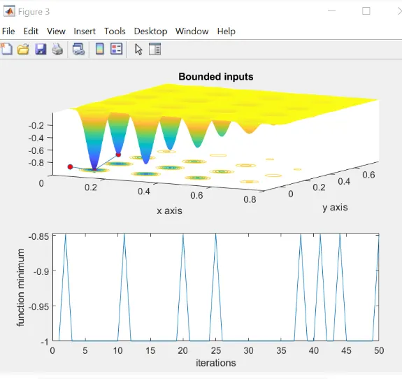
- With 600 Iterations:

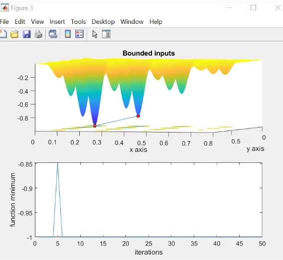
And that's it, thanks.