Week 11 - Simulation of Flow through a pipe in OpenFoam
Simulation of Flow through a pipe in OpenFoam
1. AIM
The following project is about the simulation of flow thorugh a pipe, using OpenFoam software; It will be defined the main equations to calculate the initial and boundary conditions from one point to another point of a determined pipe, then, it will be used OpenFoam in order to check the flow behavior inside the pipe and finally, using MATLAB, it will be developed a code which will update some data sheet, to also update the OpenFoam data and perform different pipe analyses.
2. EQUATIONS
Reynolds Equation
`Re=(V_(avg)rhoD)/mu`
Where:
D= pipe diameter
`rho=`fluid density
Hagen-Poiseuille's Equation
Hagen-Poiseuille's equation is the main equation to determine de drop pressure inside the pipe. This equation is used once the fully developed flow occurs:
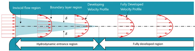
The equation will look like:
`Deltap=(8muLV_(avg))/(R^2)`
Where:
`mu`= Dynamic fluid viscosity
L= pipe length
`V_(avg)`=Average velocity when the fully developed flow is achieved.
R= pipe radius
Furthermore, OpenFoam uses the kinematic pressure in its simulations, this kinematic pressure is calculated as:
`P_k=(Deltap)/rho`
To get the appropiate length, the following equation is used:
`L_h=0.06ReD`
3. OBJECTIVES
- Define the main equations of a pipe to get the initial and boundary conditions.
- Understand the wedge boundary theorem in order to use it in the front and back pipe mesh.
- Determine the flow behavior along the pipe length using different geometry parameters.
4. ENGINEERING DEVELOPMENT
According to the challenge statements that adress this project, the diameter can be selected and the wedge angle of the front and back faces could be 5 degrees or less, knowing the wedge boundary is one kind of boundary geometry which is used to get a axi-symetric geometry on the analyzed component. This kind of geometry is used in geometries like cylinders, spheres, conical geometries, ect.
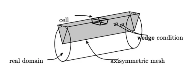
Asie, OpenFoam allows to generate this type of shapes using the sentence "wedge", so, taking into account the corner points are given by:
`._y=Rsin(alpha)`
`._z=Rcos(alpha)`
Where `alpha`is the wedge angle. And also taking into account the Reynolds number is for laminar flow and the flow is incompressible, the blockMeshDict information will be:
/--------------------------------- C++ -----------------------------------\
  =========                 |
  \\      /  F ield         | OpenFOAM: The Open Source CFD Toolbox
   \\    /   O peration     | Website:  https://openfoam.org
    \\  /    A nd           | Version:  9
     \\/     M anipulation  |
\---------------------------------------------------------------------------/
FoamFile
{
    format      ascii;
    class       dictionary;
    object      blockMeshDict;
}
// * * * * * * * * * * * * * * * * * * * * * * * * * * * * * * * * * * * * * //

convertToMeters 1;

vertices
(
    (0 0 0) //00
    (0 0.0024976206 0.0001090485) //01
    (0 0.0024976206 -0.0001090485) //02
    (2 0 0) //03
    (2 0.0024976206 0.0001090485) //04
    (2 0.0024976206 -0.0001090485) //05
);

blocks
(
    hex (0 3 5 2 0 3 4 1) (400 30 1) simpleGrading (1 0.1 1)
);

edges
(
    arc 1 2 (0 0.010 0)
    arc 4 5 (2 0.010 0)
);

boundary
(
    axis
    {
        type empty;
        faces
        (
            (0 3 3 0)
        );
    }
    inlet
    {
        type patch;
        faces
        (
            (0 1 2 0)
        );
    }
    outlet
    {
        type patch;
        faces
        (
            (3 4 5 3)
        );
    }
    front
    {
        type wedge;
        faces
        (
            (0 3 4 1)
        );
    }
    back
    {
        type wedge;
        faces
        (
            (0 2 5 3)
        );
    }

    pipewall
    {
        type wall;
        faces
        (
            (1 4 5 2)
        );
    }
);

mergePatchPairs
(
);

// *********************************************************************************//
The x axis is divided in 400 elements, y axis in 30 and z axis just in 1 element, arc is used to define the wedge radius and the position points over the OpenFoam software. Now, the controlDict is defined as:
/--------------------------------- C++ -----------------------------------\
  =========                 |
  \\      /  F ield         | OpenFOAM: The Open Source CFD Toolbox
   \\    /   O peration     | Website:  https://openfoam.org
    \\  /    A nd           | Version:  9
     \\/     M anipulation  |
\---------------------------------------------------------------------------/
FoamFile
{
    format      ascii;
    class       dictionary;
    location    "system";
    object      controlDict;
}
// * * * * * * * * * * * * * * * * * * * * * * * * * * * * * * * * * * * * * //

application     icoFoam;

startFrom       startTime;

startTime       0;

stopAt          endTime;

endTime         40;

deltaT          0.1;

writeControl    timeStep;

writeInterval   200;

purgeWrite      0;

writeFormat     ascii;

writePrecision  6;

writeCompression off;

timeFormat      general;

timePrecision   6;

runTimeModifiable true;


// ***********************************************************************************//
The step time will be 0.1 and the analysis will be from 0 to 40 seconds. Finally, the average velocity obtained was 0.08431893 (m/s) and the kinematic pressure obtained was 0.00216676. Those two values were obtained using water as the inside pipe fluid at T=25°C.
U:
/--------------------------------- C++ -----------------------------------\
  =========                 |
  \\      /  F ield         | OpenFOAM: The Open Source CFD Toolbox
   \\    /   O peration     | Website:  https://openfoam.org
    \\  /    A nd           | Version:  9
     \\/     M anipulation  |
\---------------------------------------------------------------------------/
FoamFile
{
    format      ascii;
    class       volVectorField;
    object      U;
}
// * * * * * * * * * * * * * * * * * * * * * * * * * * * * * * * * * * * * * //

dimensions      [0 1 -1 0 0 0 0];

internalField   uniform (0.08431893 0 0);

boundaryField
{
    axis
    {
        type            empty;
    }

    inlet
    {
        type            fixedValue;
        value           uniform (0.08431893 0 0);
    }

    outlet
    {
        type            zeroGradient;
    }
    front
    {
        type            wedge;
    }
    back
    {
        type            wedge;
    }
    pipewall
    {
        type            noSlip;
    }
}

// ***********************************************************************************//
p:
/--------------------------------- C++ -----------------------------------\
  =========                 |
  \\      /  F ield         | OpenFOAM: The Open Source CFD Toolbox
   \\    /   O peration     | Website:  https://openfoam.org
    \\  /    A nd           | Version:  9
     \\/     M anipulation  |
\---------------------------------------------------------------------------/
FoamFile
{
    format      ascii;
    class       volScalarField;
    object      p;
}
// * * * * * * * * * * * * * * * * * * * * * * * * * * * * * * * * * * * * * //

dimensions      [0 2 -2 0 0 0 0];

internalField   uniform 0;

boundaryField
{
    axis
    {
        type            empty;
    }

    inlet
    {
        type            zeroGradient;
    }

    outlet
    {
        type            fixedValue;
        value           uniform 0.00216676;
    }
    front
    {
        type            wedge;
    }
    back
    {
        type            wedge;
    }
    pipewall
    {
        type            zeroGradient;
    }
}

// ********************************************************************************//
The kinematic viscosity of water at 25 Celcius degrees is equal to 8.92`*10^-7`; having all this parameters the following step is to define the MATLAB code, this one is attached below as the code writting as the MATLAB sheet.
MATLAB CODE:
%Week 11 - Simulation of Flow through a pipe in OpenFoam
%Engr. Diego Alejandro Cepeda Cuartas

%In this challenge, you will simulate an axi-symmetric flow by applying the
% wedge boundary condition. The flow is laminar and flows through a constant
% cross-section pipe at an inlet Reynold's number of 2100. You can do a
% transient or steady state simulation and you will validate your results
% with the Hagen- Poiseuille's equations for the fully developed flow.

%You will also write code in Matlab to automate the generation of
% blockMeshDict file. The code should take inputs like pipe length,
% diameter, wedge angle, etc and output a fully functional blockMeshDict
% file.

%Expected Results

%Validate Hydro-dynamic length with the numerical result
%Validate the fully developed flow velocity profile with its analytical profile
%Validate maximum velocity and pressured drop for fully developed flow
%Post-process Shear stress and validate wall shear stress for fully developed flow

%Hint

%You can create a wedge from a hex block by collapsing its bottom face
% (by merging both sets of adjacent vertices)
%Wedge angle should be less than 5 degrees
%You can assume the pipe diameter

%SOLUTION:
%CODE:

clear all
close all
clc

%STEP 1. Geometry features
% Diameter of Pipe (m)
d = 0.025;

% Radius of Pipe (m)
r = d/2;

% Reynold's Number
Re = 2100;

% Wedge Angle (degrees)
theta = 5;

% Total Length of the Pipe (m)
L = 2.8;


% Assuming working fluid is water at 25° C
% Density of water (kg/m³)
rho = 998.21;

% Dynamic Viscosity of Water (Pa.s)
mu = 1.002 * 10^-3;

% Kinematic Viscosity of Water (m^2/s)
nu = mu/rho;


% Hydrodynamic Entrance Length (m)
L_h = 0.06 * Re * D;


% STEP 2. Initial & Boundary conditions
% Hagen - Pousielle's flow equation
V_avg = (mu * Re)/(rho * D); % Average Velocity (m/s)

V_max = 2 * V_avg; % Maximum Velocity (m/s)

delta_p = (32*mu*V_avg*L)/(D^2); % Pressure Drop (Pa)

kinematic_delta_p = delta_p/rho; % Kinematic Pressure Drop (Pa)

% STEP 3. Defining OpenFoam requirements

% Vertices
V0 = [0 0 0];
V1 = [0 R*cosd(theta/2) -R*sind(theta/2)];
V2 = [0 R*cosd(theta/2) R*sind(theta/2)];

V3 = [L 0 0];
V4 = [L R*cosd(theta/2) -R*sind(theta/2)];
V5 = [L R*cosd(theta/2) R*sind(theta/2)];


% BLOCKMESHDICT FILE
% Creating the file
% Header
h1 = '/*--------------------------------*- C++ -*----------------------------------*\';
h2 = '  =========                 |';
h3 = '  \\      /  F ield         | OpenFOAM: The Open Source CFD Toolbox';
h4 = '   \\    /   O peration     | Website:  https://openfoam.org';
h5 = '    \\  /    A nd           | Version:  9';
h6 = '     \\/     M anipulation  |';
h7 = '\*---------------------------------------------------------------------------*/';
h8 = 'FoamFile';
h9 = '{';
h10 = '    format      ascii;';
h11 = '    class       dictionary;';
h12 = '    object      blockMeshDict;';
h13 = '}';
h14 = '// * * * * * * * * * * * * * * * * * * * * * * * * * * * * * * * * * * * * * //';


% Creating BlockMesh File
f1 = fopen('blockMeshDict.txt','w');

% Header
fprintf(f1,'%s\n',h1);
fprintf(f1,'%s\n',h2);
fprintf(f1,'%s\n',h3);
fprintf(f1,'%s\n',h4);
fprintf(f1,'%s\n',h5);
fprintf(f1,'%s\n',h6);
fprintf(f1,'%s\n',h7);
fprintf(f1,'%s\n',h8);
fprintf(f1,'%s\n',h9);
fprintf(f1,'%s\n',h10);
fprintf(f1,'%s\n',h11);
fprintf(f1,'%s\n',h12);
fprintf(f1,'%s\n',h13);
fprintf(f1,'%s\n\n',h14);

% Conversion Factor
fprintf(f1,'%s\n\n','convertToMeters 1;');

% Vertices
fprintf(f1,'%s\n','vertices');
fprintf(f1,'%s\n','(');
fprintf(f1,'\t(%d %d %d)\n',V0);
fprintf(f1,'\t(%d %f %f)\n',V1);
fprintf(f1,'\t(%d %f %f)\n',V2);
fprintf(f1,'\t(%.2f %d %d)\n',V3);
fprintf(f1,'\t(%.2f %f %f)\n',V4);
fprintf(f1,'\t(%.2f %f %f)\n',V5);
fprintf(f1,'%s\n\n',');');

% Blocks
fprintf(f1,'%s\n','blocks');
fprintf(f1,'%s\n','(');
fprintf(f1,'\thex (0 3 4 1 0 3 5 2) (400 30 1) simpleGrading (1 0.1 1)\n');
fprintf(f1,'%s\n\n',');');

% Edges
fprintf(f1,'%s\n','edges');
fprintf(f1,'%s\n','(');
fprintf(f1,'\tarc 2 1 (%d %.3f %d)\n',0,R,0);
fprintf(f1,'\tarc 5 4 (%.3f %.3f %d)\n',L,R,0);
fprintf(f1,'%s\n\n',');');

% Boundary
fprintf(f1,'%s\n','boundary');
fprintf(f1,'%s\n','(');

% Axis
fprintf(f1,'\taxis\n');
fprintf(f1,'\t{\n');
fprintf(f1,'\t\ttype empty;\n');
fprintf(f1,'\t\tfaces\n');
fprintf(f1,'\t\t(\n');
fprintf(f1,'\t\t\t(0 3 3 0)\n');
fprintf(f1,'\t\t);\n');
fprintf(f1,'\t}\n\n');

% Inlet
fprintf(f1,'\tinlet\n');
fprintf(f1,'\t{\n');
fprintf(f1,'\t\ttype patch;\n');
fprintf(f1,'\t\tfaces\n');
fprintf(f1,'\t\t(\n');
fprintf(f1,'\t\t\t(0 1 2 0)\n');
fprintf(f1,'\t\t);\n');
fprintf(f1,'\t}\n\n');

% Outlet
fprintf(f1,'\toutlet\n');
fprintf(f1,'\t{\n');
fprintf(f1,'\t\ttype patch;\n');
fprintf(f1,'\t\tfaces\n');
fprintf(f1,'\t\t(\n');
fprintf(f1,'\t\t\t(3 5 4 3)\n');
fprintf(f1,'\t\t);\n');
fprintf(f1,'\t}\n\n');

% Front Face
fprintf(f1,'\tfront\n');
fprintf(f1,'\t{\n');
fprintf(f1,'\t\ttype wedge;\n');
fprintf(f1,'\t\tfaces\n');
fprintf(f1,'\t\t(\n');
fprintf(f1,'\t\t\t(0 3 4 1)\n');
fprintf(f1,'\t\t);\n');
fprintf(f1,'\t}\n\n');

% Back Face
fprintf(f1,'\tback\n');
fprintf(f1,'\t{\n');
fprintf(f1,'\t\ttype wedge;\n');
fprintf(f1,'\t\tfaces\n');
fprintf(f1,'\t\t(\n');
fprintf(f1,'\t\t\t(0 2 5 3)\n');
fprintf(f1,'\t\t);\n');
fprintf(f1,'\t}\n\n');

% Top Wall
fprintf(f1,'\tpipeWall\n');
fprintf(f1,'\t{\n');
fprintf(f1,'\t\ttype wall;\n');
fprintf(f1,'\t\tfaces\n');
fprintf(f1,'\t\t(\n');
fprintf(f1,'\t\t\t(1 4 5 2)\n');
fprintf(f1,'\t\t);\n');
fprintf(f1,'\t}\n');

fprintf(f1,'%s\n\n',');');
fprintf(f1,'%s\n','mergePatchPairs');
fprintf(f1,'%s\n','(');
fprintf(f1,'%s\n\n',');');
fprintf(f1,'%s\n','// ************************************************************************* //');
5. RESULTS
Geometry
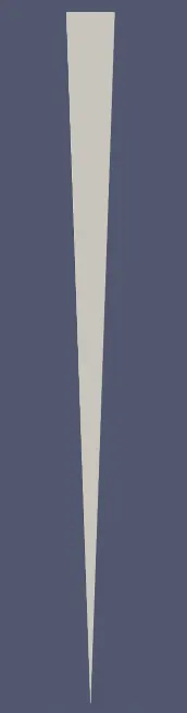
The geometry obtained on the cross section looks like:
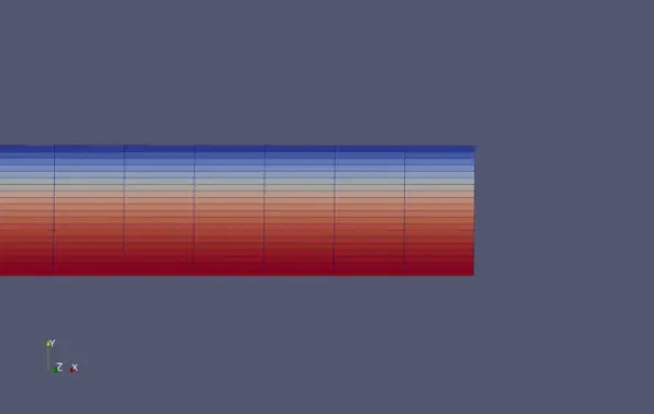
And the mesh along the pipe:
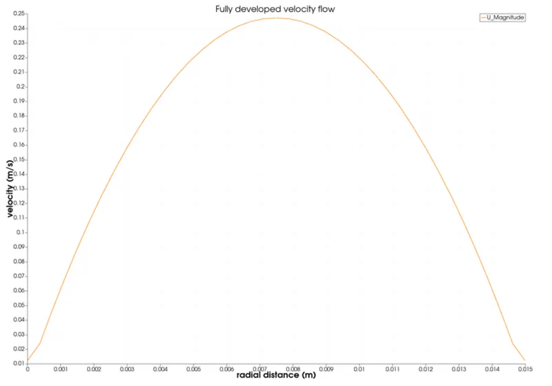
The fully developed flow is obtained between L=0.5m and L=2m, so, the velocity profile along these sections will be:
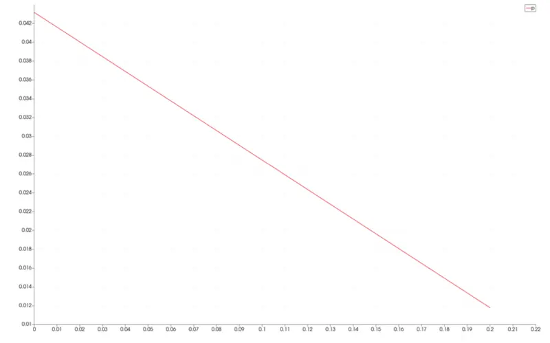
Likewise the pressure drop is getting down along the length in a correct form, and the line slope should be eual to the result obtained in the Hagen-Poiseuille's equation.
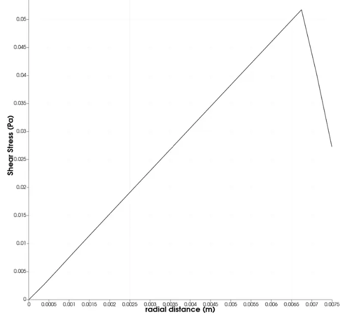
Also, looking at the cross section, the shear stress along the pipe is higher at the pipe walls than the center inner pipe.
Finally, comparing the numerical results with the analytical results obtained, it can be seen the velocity and pressure along the wall behaves similar win the both methods.
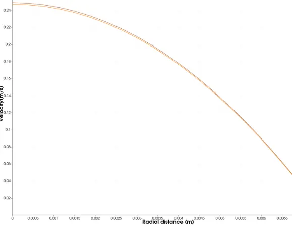
The red line is about the numerical method and the yellow about the analytical method.
6. CONCLUSIONS
Numerical method in OpenFoam approximates the flow behavior very similar to the analytical method and, generates high quality plots that shows the real behavior inside the objects. Due to that, OpenFoam is a good key to simulate CFD problems which to require the inner analysis of flows through different objects.
One of the bad disadvantage of OpenFoam is the way that the data must be updated, due to this issue, MATLAB gets easily the way to update the new data, so, if the user is clearly about the method he needs to use, he will just have to generate a MATLAB code that updates the OpenFoam sheets faster.
That's it, thanks for reading.
7. REFERENCES
https://doc.cfd.direct/notes/cfd-general-principles/axisymmetric-wedge-condition