Week 7 - CHT Analysis on a Graphics card

                                   CHT Analysis on a graphic card - Final project

AIM

The following project is about a Conjugate Heat Transfer (CHT) analysis over a commercial graphic card used in different electronic devices. CHT is a thermal analysis method huge used in different industries as coolers manufacturers, mechanical designs, engines analyses, etc. And the importance of this method is because of it can be simultaniously simulated the thermal behavior of solid and fluid materials interacting in a encluosed space. 

In this project will be firstly refined the mesh which will be put on the graphic card geometry, using different mesh refinement methods and then, it will be simulated the flow behavior using three different velocities, in order to watch what it happens with the heat transfer coefficient on the components when it is dived under a flow field. Finally, it will be plotted and explained the results obtained, comparing each simulation result.

EQUATIONS

Heat volumetric source= `Q/V`

Where:

Q= rate which the heat is transferred

V= is the object volume

OBJECTIVES

Simulate the flow movement around a conventional graphic card with an specific geometry, by means of ANSYS Fluent.

Determine the maximum temperature and the average heat transfer coefficient in the processer component from the graphic card. 

Explain the results obtained in each simulation along with the contour plots obtained.

ENGINEERING DEVELOPMENT

It is firstly updated the component geometry provided by the challenge statements and then, it is used share tool in SpaceClaim to make sure the mesh elements will fit each other in every component boundary where two components have been joint, including the mesh which will play as a fluid in the simulation. The main components of the geometry are:

• Base

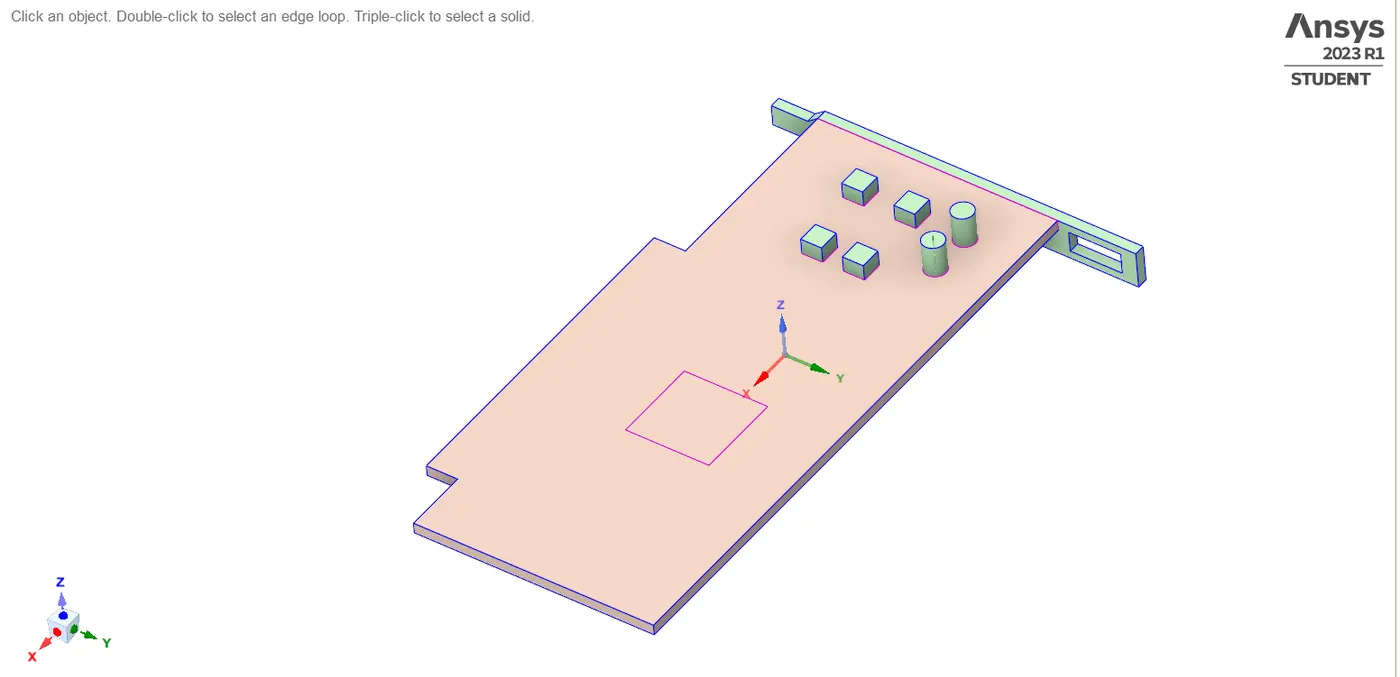
• Processer

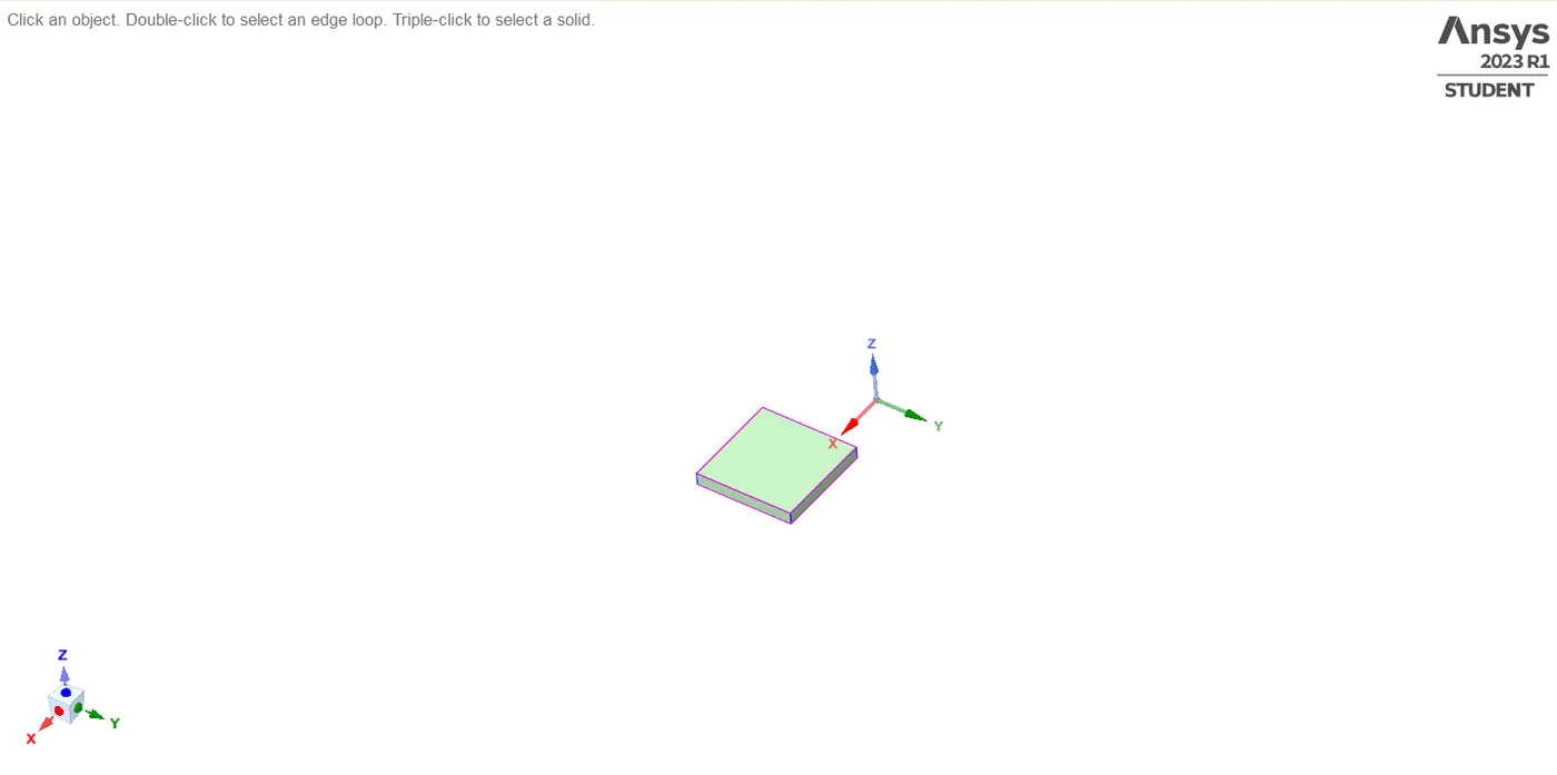
• Fins

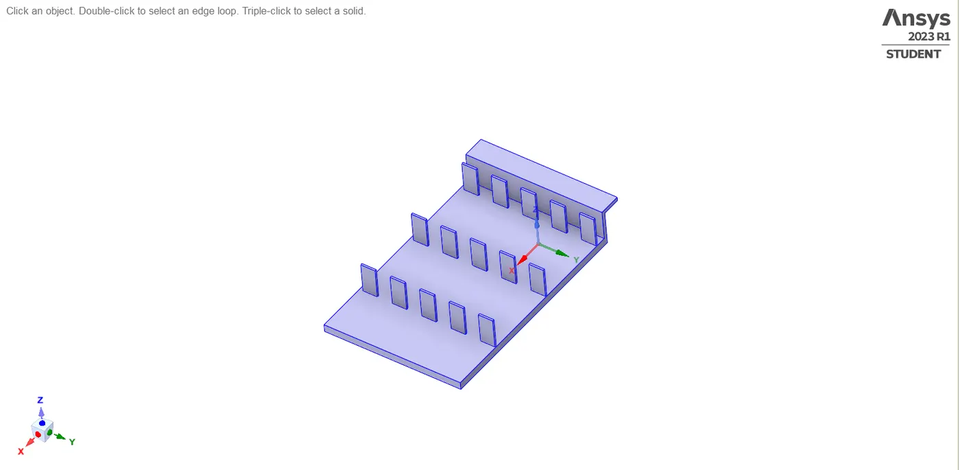
• Enclosure

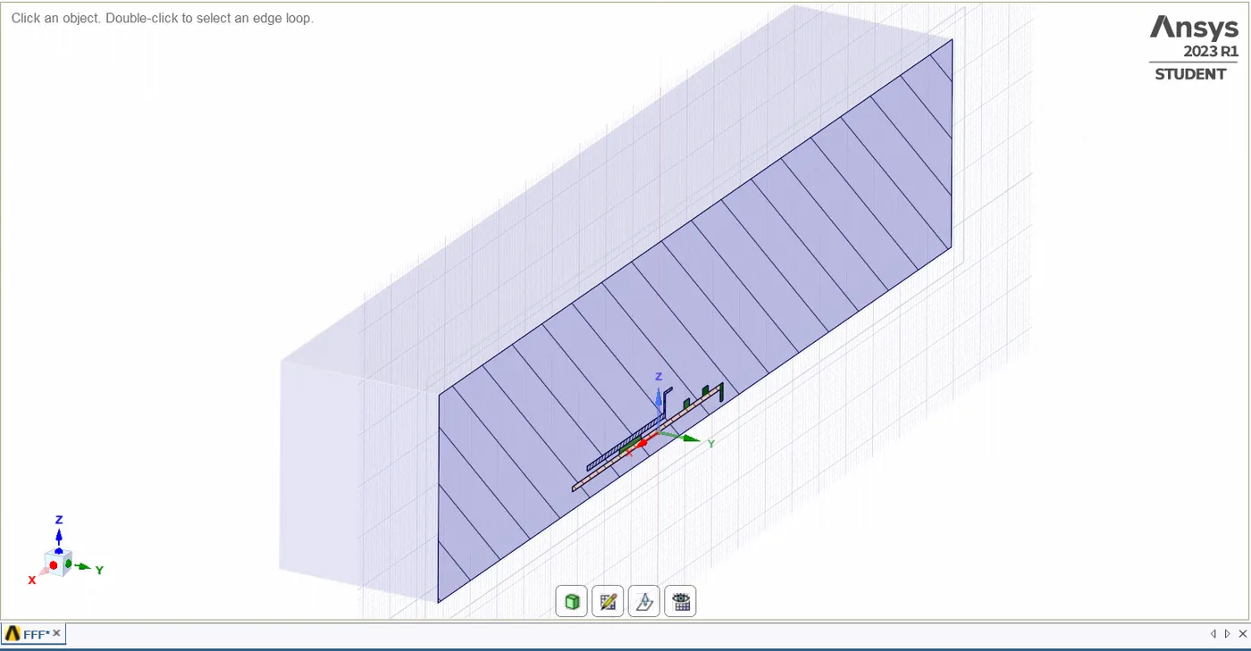
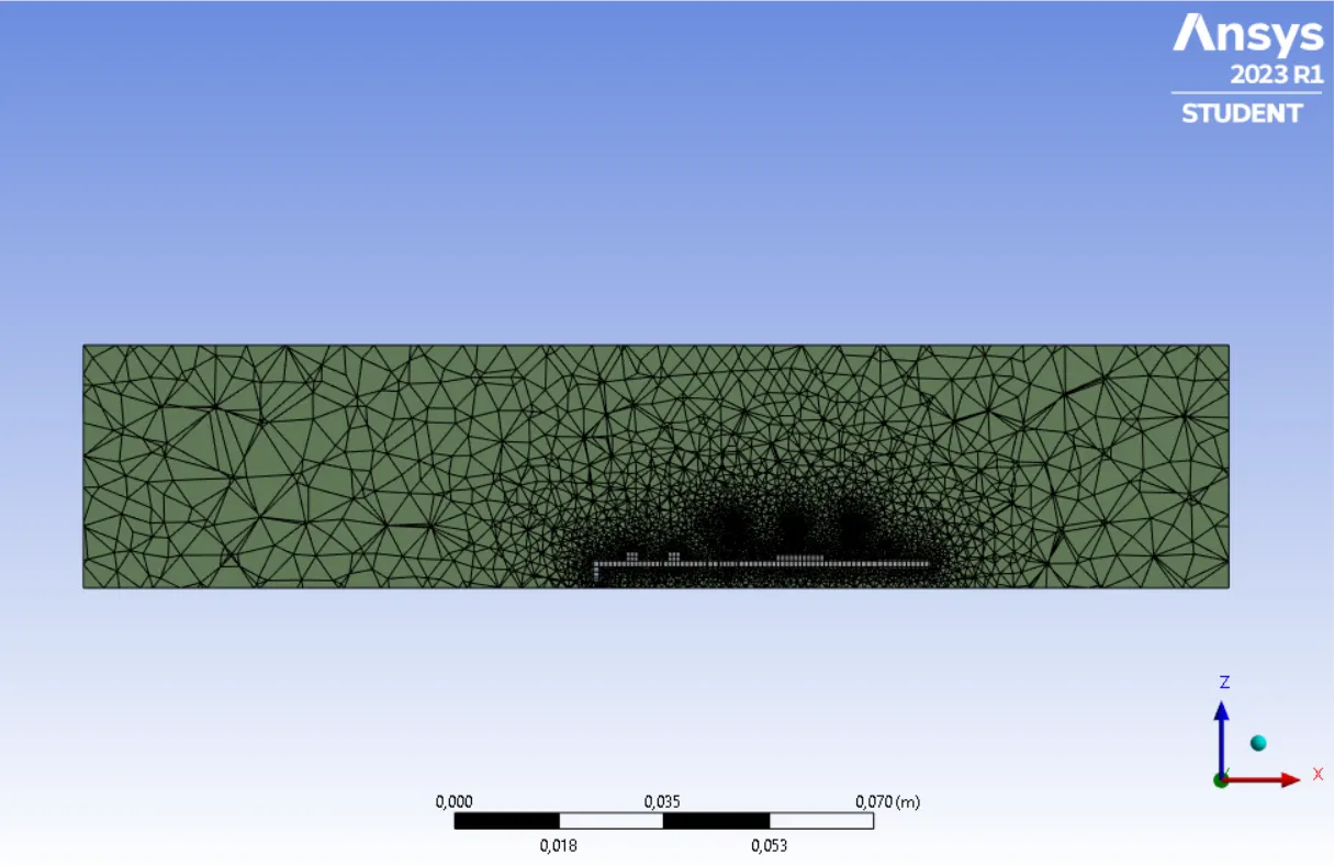
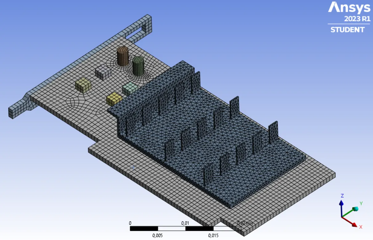
To show the enclosure component clearer, it was cut on the middle; in the picture above it can be seen the graphic components into the enclosure domain. Once the share tool is ran up and there is any single error in the geometry refinement, the geometry mesh is generated and the mesh over each component is refined. Using mesh refinement methods , the mesh size over each component will be equal to:

Component	Element size (m)
Fins	0.00075
Processer	0.0075
Base	0.00075
Enclosure	0.0075

The reason of using this type of refinement in each component is due to the main results that are seeked here, are in the inner sections from the graphic card components, being necessary a mesh which will get accurate results; also, the processer element sizes are not refined due to its mesh refinement occurs automatically once the external components are refined too. This refinement process is thanks to the low thickness that the processer component has. The final component mesh will look as is shown in the pictures above.

• Final general fmesh refinement 

• Final graphic card mesh refinement

Now, the simulation can be carried out, it will be used three different flow velocity magnitude, in order to see the heat transfer coefficient variation in each flow field. Furthermore, according to different researches, it is normal the processer and the graphic card in general generate a heat transfer rate of 50W when this one is working. Thus, the primitive parameters used in each simulation will be:

Cases	Flow velocity (m/s)	Processer heat transfer rate (W)
I	1	50
II	3	50
III	5	50

Heat volumetric source=`(50W)/(64*10^-6m^3)`= 781125000`W/(m^3)`

• Case I:

SETUP
Solver Type	Pressure-Based
Velocity Formulation	Absolute
Time	Steady
Models	Viscous model: K-omega SST Energy model: On
Material	Fluid type: Air  Solid-type: Aluminium                : Titanium                : Steel
Cell zones	Fluid type: Air  Solid: Ti, Ti, Steel
Boundaries	Inlet : inlet velocity: 1 m/s         : temperature = 288K Outlet: outlet pressure = 0
Reference values	Standard
Initialization	Hybrid

• Case II:

SETUP
Solver Type	Pressure-Based
Velocity Formulation	Absolute
Time	Steady
Models	Viscous model: K-omega SST Energy model: On
Material	Fluid type: Air  Solid-type: Aluminium                : Titanium                : Steel
Cell zones	Fluid type: Air  Solid: Ti, Ti, Steel
Boundaries	Inlet : inlet velocity: 3 m/s         : temperature = 288K Outlet: outlet pressure = 0
Reference values	Standard
Initialization	Hybrid

• Case III:

SETUP
Solver Type	Pressure-Based
Velocity Formulation	Absolute
Time	Steady
Models	Viscous model: K-omega SST Energy model: On
Material	Fluid type: Air  Solid-type: Aluminium                : Titanium                : Steel
Cell zones	Fluid type: Air  Solid: Ti, Ti, Steel
Boundaries	Inlet : inlet velocity: 5 m/s         : temperature = 288K Outlet: outlet pressure = 0
Reference values	Standard
Initialization	Hybrid

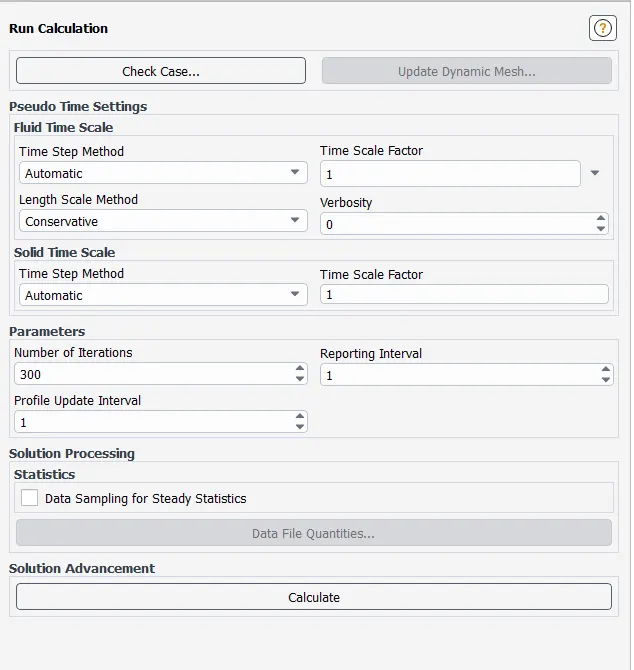
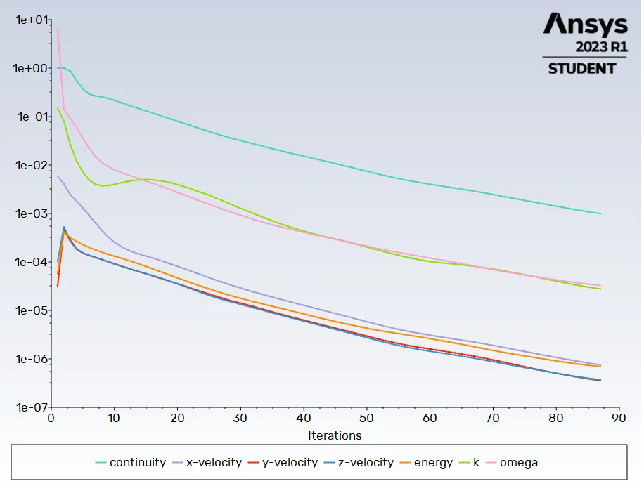
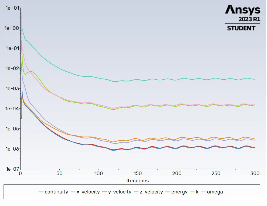
The calculation is ran-up using 300 iterations, however, `k-omega` model can find the convergency in a less amount of iterations.

RESUTLS

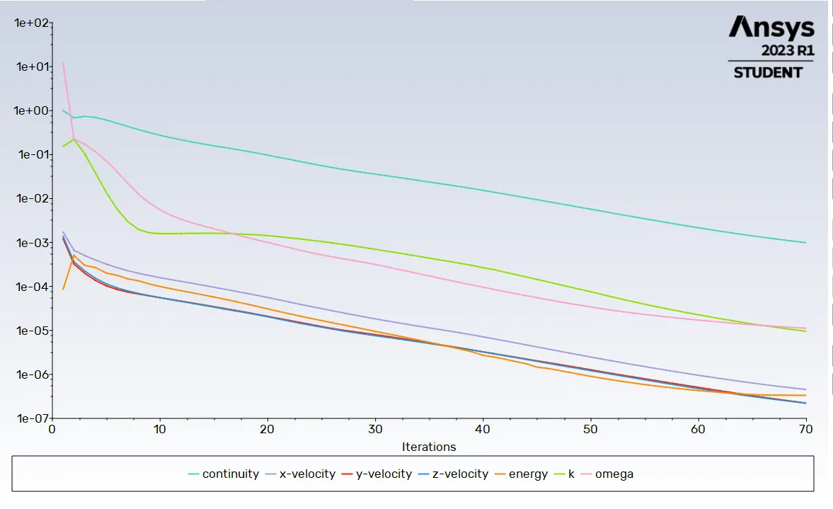
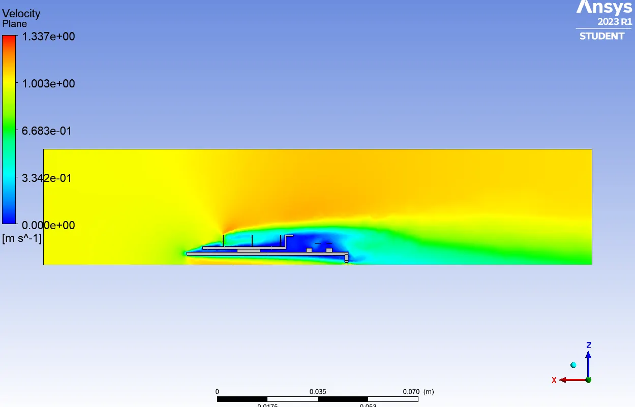
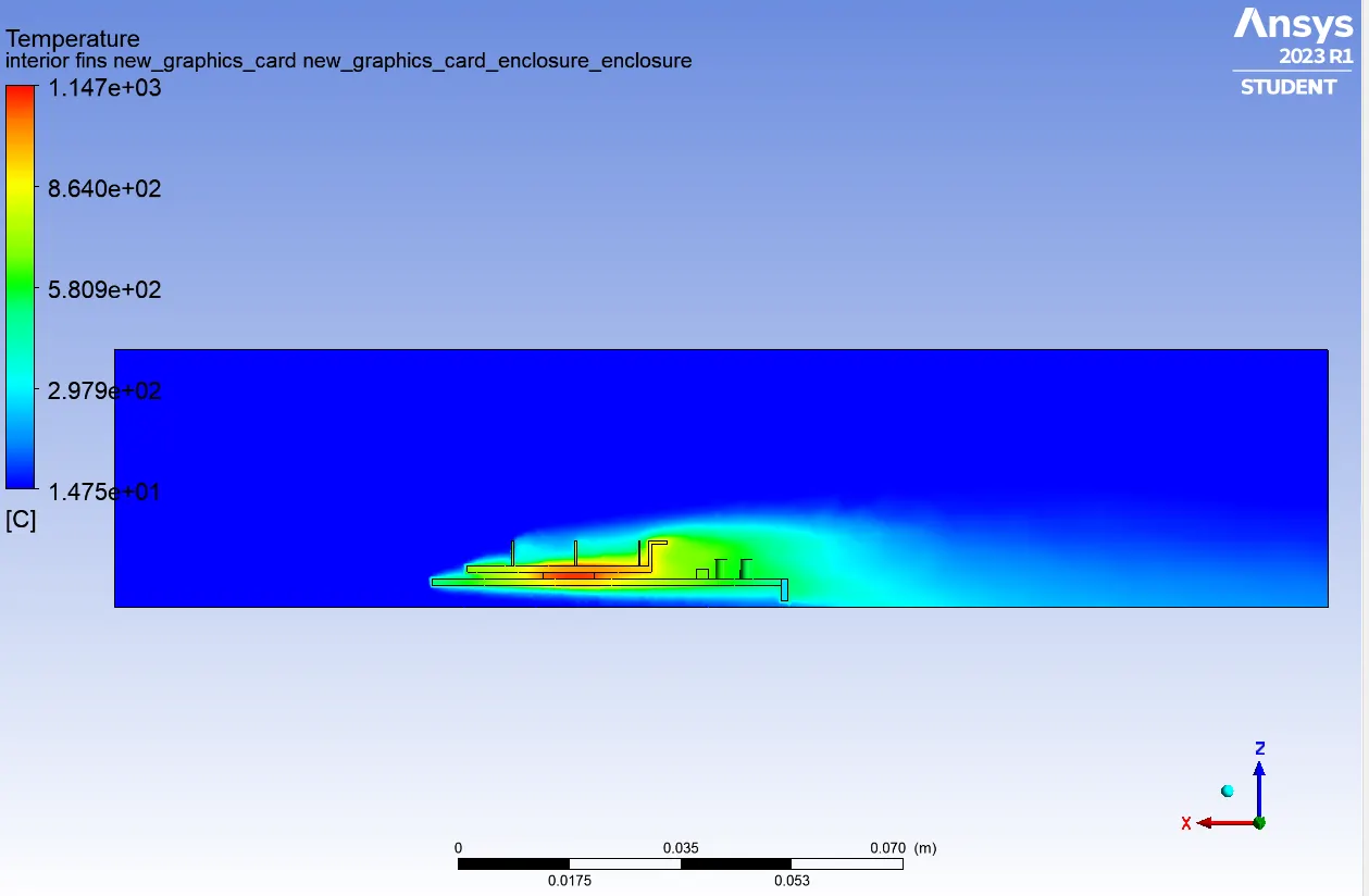
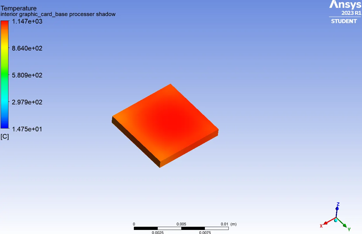
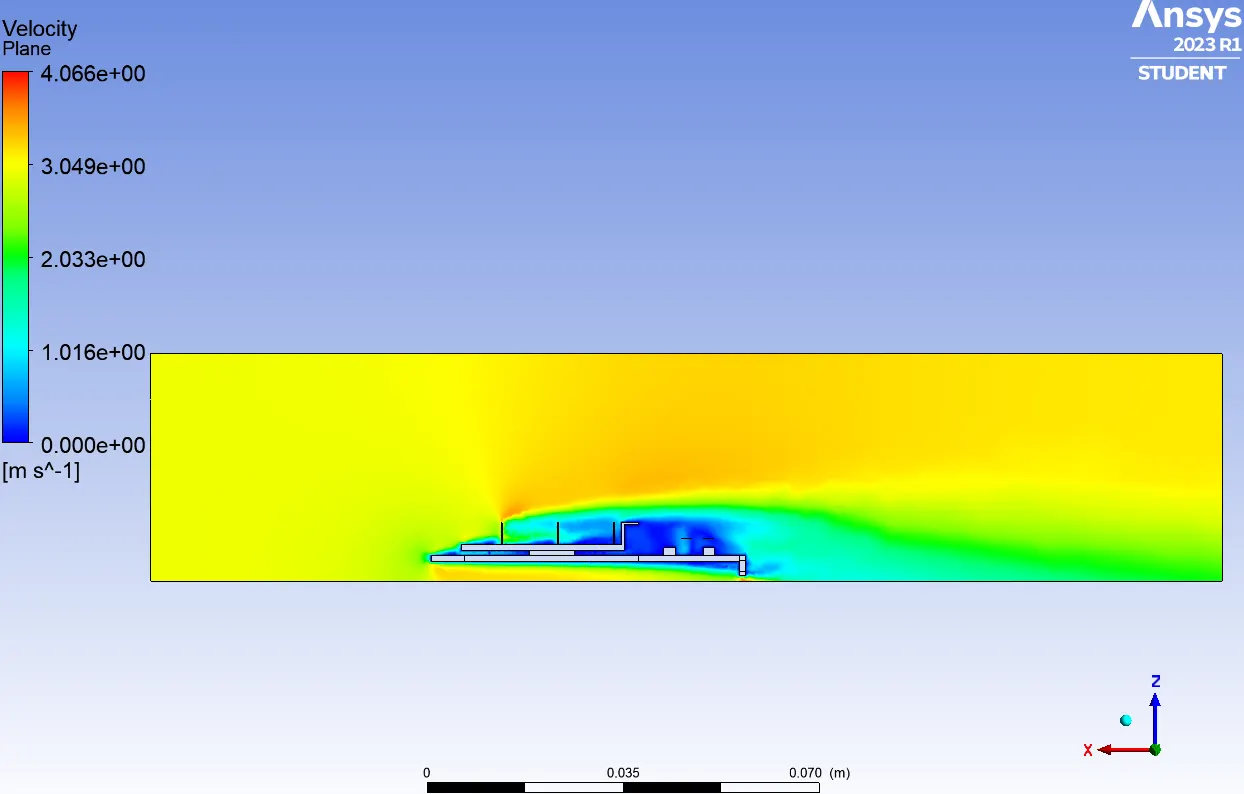
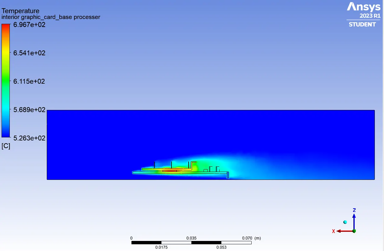
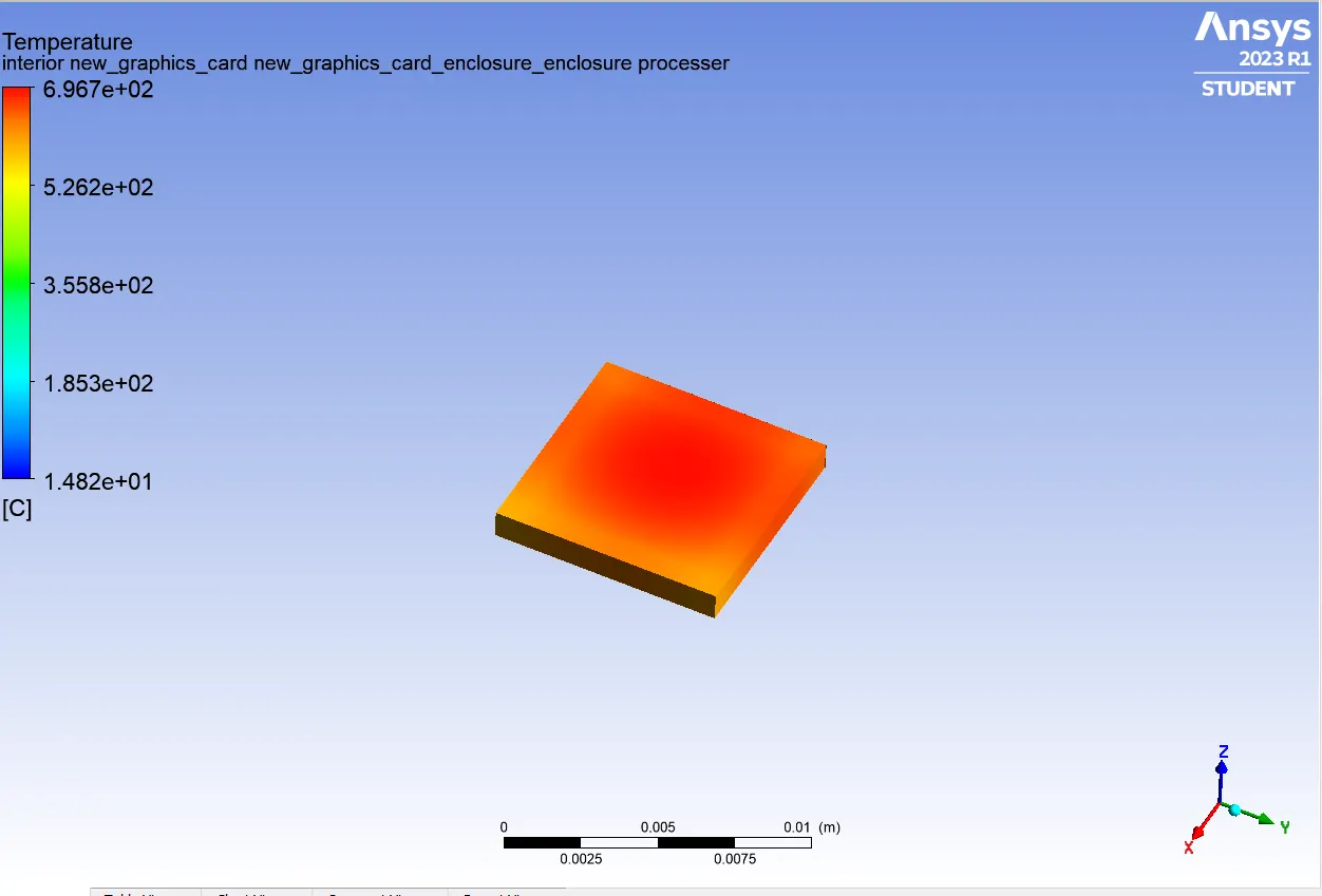
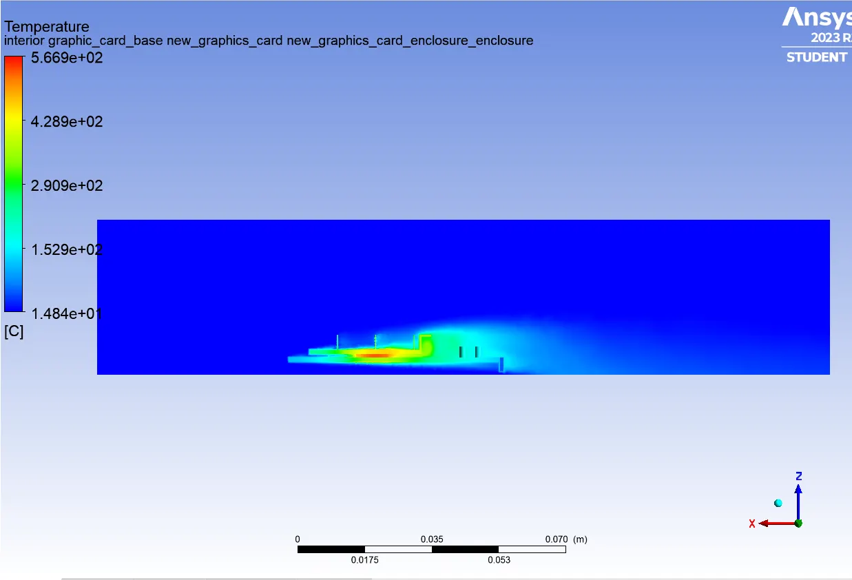
The results obtained in each case are attached below. Convergency plot, Velocity contour, Temperature contour and temperature gradient around the processer component are shown in each case. It can be seen just the last case does not get the convergency as quick as the other ones.

Case I:

• Convergency

• Velocity

• Temperature

• Processer temperature gradient

Case II:

• Convergency

• Velocity

• Temperature

• Processer temperature gradient

Case III:

• Convergency

• Velocity

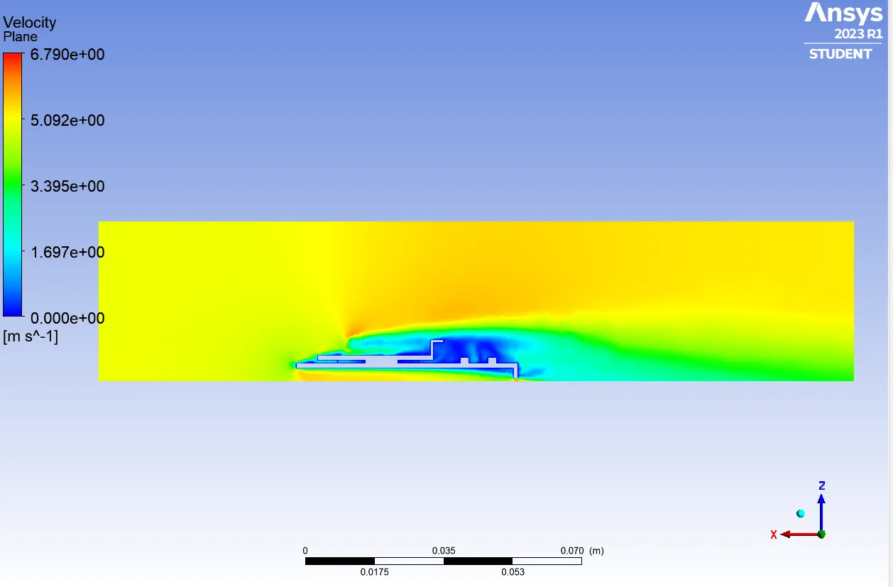
• Temperature

• Processer temperature gradient

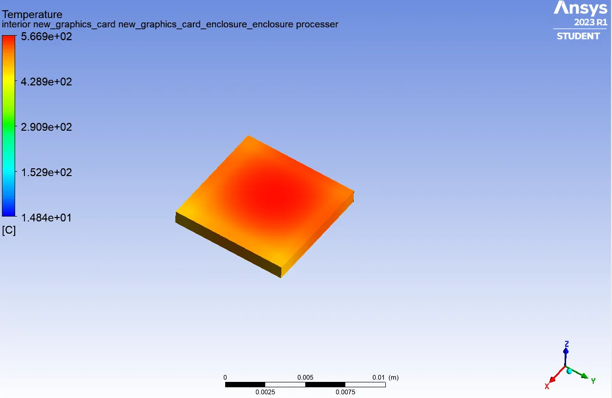
Likewise, the maximum temperature over the processer component which is the main component who is analyzed in all the simulations, is shown in the table below along with the average heat transfer coefficient that the program computed for each case.

Cases	Flow velocity (`m/s`)	Maximum temperature (K)	Heat transfer coefficient (`W/(m^2K)`)	% of variation
I	1	1406	361.77	N/A (Starting point)
II	3	962	361.9	0.036
III	5	832	362.11	0.094

The hottest spots in the model are found in the middle of the component, in each case is shown the red zone represents the hottest points and it is always in the middle.

CONCLUSIONS

The simulation was successful and it can be certainly assumed due to the heat transfer coefficient does not get high variations from the first case to another one. However, it is a little complex to get an initial value by calculating the average transfer coefficient in a paper sheet, due to the thermal conductive and the areas where the thermal conductive of any object is working make the average heat transfer analysis becomes difficult of getting.

It cannot be used `Y+`in the model due to the components were small enough, such that the total turbulent layer was even bigger than the thickness of two components.

Fins are commonly used in the industry to generate a forced convective transfer which the internal zones from any component reach a desired hotting or cooling, depending on the industry requirement. But, because of the heat transfer along them is not alike along their heigth, it has to be carried out a temperature handling whereby the fins reach their desired operational features. ANSYS get easier the fin heat transfer calculation, however, it must be taken into account some references researches which make sure the results obtained are correct.

REFERENCES

www.me.psu.edu/cimbala/me433/Links/Table_A_9_CC_Properties_of_Air.pdf 

www.mhtl.uwaterloo.ca/courses/ece309_mechatronics/lectures/pdffiles/chapter6.pdf

 https://byjus.com/physics/heat-transfer-convection/ 

https://iaeme.com/MasterAdmin/Journal_uploads/IJMET/VOLUME_11_ISSUE_2/IJMET_11_02_002.pdf