Week 3 - Solving second order ODEs

1. Pendulum Damping Movement Simulation - Behavior Code:

%Pendulum Damping Movement Simulation 
%Diego Alejandro Cepeda Cuartas
clear all
clc

%Sysmtem Parameters
L=1 %String Lenght (m)
m=1 %Sphere Mass (Kg)
b=0.05 %Damping (N/m)
g=9.81 %Gravity acceleration(m/s^2)

%Initial parameters 
theta_o=[0;3] %[Displacement,angular velocity]

%Time points between 20 seconds
t_span=linspace(0,20,500)

%Equation solution by ode45 function 
[t,results]=ode45(@(t,theta_value) ODE_solution(t ,theta_value ,L,m,b,g),t_span,theta_o)

%Plot results for theta 1 and theta 2 
hold on
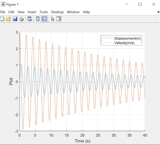
plot(t,results(:,1)) %Displacement Plot
plot(t,results(:,2)) %Velocity Plot
xlabel('Time (s)')
ylabel('Plot')
legend('Displacement(m)','Velocity(m/s)')
grid on

2. Pendulum Damping Movement Simulation - Iteration Function Code:

function [Theta]=ODE_solution(t,theta_value,L,m,b,g)
theta_1=theta_value(1);
theta_2=theta_value(2);
dtheta1_dt=theta_2;
dtheta2_dt=-(b/m)*theta_2-(g/L)*sin(theta_1);
Theta=[dtheta1_dt;dtheta2_dt];
end

3. Pendulum Damping Movement Simulation- Pendulum Displacement Simulation Code:

%Pendulum Displacement Simulation 
theta=rad2deg(results(:,1))
ct=1

%For loop 
for i=1:length(theta)
    n=theta(i)
    
    %Ground point
    xo=0
    yo=0 
    
    %String Length
    L1=1
    
    %x and y position equations
    x1=L1*sind(n)
    y1=-L1*cosd(n)
    
    %Dynamic chart
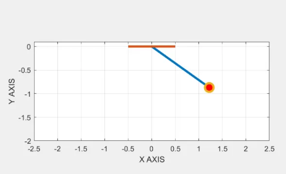
    plot([xo x1],[yo y1],[-0.5 0.5],[0 0],x1,y1,'-o',...
        'MarkerSize',12,...
        'MarkerFaceColor','r',...
        'linewidth',3)
    axis equal
    axis([-2.5 2.5 -2 0.1])
    xlabel('X AXIS')
    ylabel('Y AXIS')
    grid on 
    pause(0.2)
    
    %Movie
    M(ct)=getframe(gcf)
    
    %Counter
    ct=ct+1
end 
movie(M)
videofile=VideoWriter('pendulum_animation.avi','Uncompressed AVI')
open(videofile)
writeVideo(videofile,M)
close(videofile)

(a)Displacement and velocity response and (b)Pendulum simulation plots:

Solving Second ODEs Report- Google Drive Link:

https://docs.google.com/document/d/1ntaFikbT-Pi5cpU4CO2nK_4a9_P20rifwbHftTwP1W8/edit?usp=sharing

Pendulum Displacement Simulation- Youtube Link:

https://www.youtube.com/watch?v=9UNTURoz1dg