Week 7 - Simulation of a 1D Supersonic nozzle flow simulation using Macormack Method

1D Supersonic Nozzle Flow Simulation using Macormack Method

1. AIM

The following project is about the 1D supersonic nozzle flow simulation using Macormack's method to solve different partial differential equations; it will be defined the main nozzle flow equations as in conservative form as in non conservative form, then, each equation will be assesed by means of Taylor series approximation equations along with the Macormack tecnique and MATLAB software, in order to check how the nozzle flow behaves regarding the time steps; finally, the different physical parameters obtained will be plotted to show the results obtained along the nozzle length and determine the the difference between conservative and non-conservative form.

2. EQUATIONS

The governing flow equations to simulate the primivite variables into a nozzle is given by the continuity equation:

`(partial)/(partialt)intintintrhodV+underset(S)(intint)rhoVdA=0`

Taking the theorem shown below and solving the continuity equation step by step with this assumption, it will get the following governing flow equations as conservative as non-conservative form.

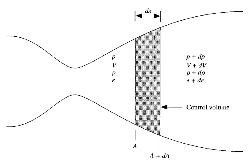
The equations obtained by solving the continuity equation are:

2.1. CONSRVATIVE FORM - GOVERNING FLOW EQUATIONS

• Continuity:

`(partial(rhoA))/(partialt)+(partial(rhoAV))/(partialx)=0`

• Momentum:

`(partial(rhoAV))/(partialt)+(partial(rhoV^2A))/(partialx)=-A(partialP)/(partialx)`

• Energy:

`(partial(rhoeA))/(partialt)+(partial(rhoeVA))/(partialx)=-P(partial(AV))/(partialx)`

2.2 NON-CONSERVATIVE FORM - GOVERNING FLOW EQUATIONS

• Continuity:

`(partial(rhoA))/(partialt)+rhoA(partialV)/(partialx)+rhoV(partialA)/(partialx)+AV(partialrho)/(partialx)=0`

• Momentum:

`rho(partialV)/(partialt)+rhoV(partialV)/(partialx)=-(partialP)/(partialx)`

• Energy:

`rho(partiale)/(partialt)+rhoV(partiale)/(partialx)=P(partialV)/(partialx)-PV(partial(lnA))/(partialx)`

3. OBJECTIVES

• Determine the PD equations for 1D supersonic nozzle flow along with its initial and boundary conditions as in conservative form as in non-conservative form.
• Perfom a MATLAB code to solve the PDE for 1D supersonic nozzle flow passing through the nozzle shape regarding each time step.
• Analyze the conservative form and non-conservative form results obtained by the MATLAB code simulation.

4. ENGINEERING DEVELOPMENT

Iteration methods normally uses different ways to reach the solutions and, to equation solution for multiple variables, it is often used the non-dimensional variables, which will indicate only how one parameter differs from a fixed parameter (the boundary value) ,dividing determined parameter over the constant parmeter located into the control volume. In the equations shown above, each parameter will be taken as:

`rho'=rho/rho_o` Density ratio

`T'=T/T_o` Temperature ratio

`P'=P/P_o` Pressure ratio

`A'=A/A^**` Area ratio regarding the nozzle throat area

`V'=V/a_o` Velocity ratio

`x'=x/L` Nozzle length

`t'=t/(L//a_o)` time ratio

Using those parameters into each equation and solving the equations in order to calculate the change of density, velocity and temperature regarding the change of time, the governing flow equations are now:

• Conservative form:

Continuity:

`(partial(rho'A'))/(partialt')=-(partial(rho'A'V'))/(partialx')`

Momentum:

`(partial(rho'A'V'))/(partialt')=-(partial(rho'V'^2A'))/(partialx')-A'(partial(Rrho'T'))/(partialx')`

Energy:

`(partial(rho'e'A'))/(partialt')=-(partial(rho'e'V'A))/(partialx')-(Rrho'T')(partial(A'V'))/(partialx')`

• Non-conservative form:

Continuity:

`(partial(rho'A'))/(partialt')=-rho'A'(partialV')/(partialx')-rho'V'(partialA')/(partialx')-A'V'(partialrho')/(partialx')`

Momentum:

`rho'(partialV')/(partialt')=-rho'V'(partialV')/(partialx')-(partial(rho'T'))/(partialx')`

Energy:

`rho'(partiale')/(partialt')=-rho'V'(partiale')/(partialx')-(Rrho'T')(partialV')/(partialx')-V'(rho'T')(partial(lnA'))/(partialx')`

Also, energy can be expressed as`e'=c_vT' and, due to the quantity of parameters that the conservative form equations have in each term, these will be simplified as:

`U1=rho'A'`

`U2=rho'V'A'=V'U1`

`U3=rho'((e')/(gamma-1)-(gamma/2)(V')^2)A'`

`F1=rho'A'V'`

`F2=rho'A'V'^2+(1/gamma)(rho'T')A'`

`F3=rho'((e')/(gamma-1)+(gamma/2)V'^2)V'A'+(rho'T')A'V'`

So, the final equations entering the energy term into each equation and converting each equation as a Taylor approximation equation, will be:

• Conservative form:

`(partialU1)/(partialt')=-(F1(i)-F1(i-1))/(Deltax)`

Momentum:

`(partialU2)/(partialt')=-(F2(i)-F2(i-1))/(Deltax)-(J2(i)-J2(i-1))/(Deltax)`

Energy:

`(partialU3)/(partialt')=-(F3(i)-F3(i-1))/(Deltax)`

• Non-conservative form:

Continuity:

`(partialrho')/(partialt')=-rho'(V'(i)-V'(i-1))/(Deltax)-rho'V'(ln(A'(i))-ln(A'(i-1)))/(Deltax)-V'(rho'(i)-rho'(i-1))/(Deltax)`

Momentum:

`(partialV')/(partialt')=-V'(V'(i)-V'(i-1))/(Deltax)-(1/gamma)((T'(i)-T'(i-1))/(Deltax)+(T')/(rho')(rho'(i)-rho'(i-1))/(Deltax))`

Energy:

`(partialT')/(partialt')=-V'(T'(i)-T'(i-1))/(Deltax')-(gamma-1)[(V'(i)-V'(i-1))/(Deltax')-V'T'(ln(A'(i))-ln(A'(i-1)))/(Deltax')]`

`gamma` is going to be equal to 1.4 and `Deltax` equal to x'/31 knowing x' is distributed from 0 to 3.

MACORMACK TECNIQUE

Macormack tecnique stipulates the following equation:

MAIN MATLAB CODE:

%Week 7 -  Simulation of a 1D Supersonic nozzle flow simulation using Macormack Method
%Engr. Diego Alejandro Cepeda Cuartas

%In this challenge you are going to simulate the isentropic flow through a 
%quasi 1D subsonic-supersonic nozzle. You will derive both the conservation 
%and non-conservation forms of the governing equations and sovle them using 
%the [MacCormack's technique. You need to determine the steady-state 
%temperature distribution for the flow-field variables and investigate 
%the difference between the two forms of governing equations by comparing 
%their solutions.


%You need to show the following plots inside your report
%1. Steady-state distribution of primitive variables inside the nozzle
%2. Time-wise variation of the primitive variables
%3. Variation of Mass flow rate distribution inside the nozzle at different 
% time steps during the time-marching process

%4. Comparison of Normalized mass flow rate distributions of both forms

%Expected Results:

%Perform a grid independence test on the solution and expain all your findings.
%The code must be modular. You need to write separate functions to solve 
%both forms.
%Discuss all the plots you are providing with observed inferences.  

%Note:
%Refer CFD book by John Anderson for Initial and boundary conditions. 

%SOLUTION:
%CODE:
close all
clear all
clc

%STEP 1. Defining the nozzle convergence-divergence flow equations.
%The flow through the nozzle varies its features regarding the length of 
%the nozzle, due to the nozzle geometry which firstly decreases and in a
%determined x point, the cross-section geometry nozzle begins to increase.
%The fundamental equations are: 

%rho1*V1*A1=rho2*V2*A2  => Mass conservation
%P1*A1+rho1*(V1^2)*A1+(P*dA)=P2*A2+rho2*(V2^2)*A2 => Momentum conservation
%h1+(V1^2)/2=h2+(V2^2)/2 => Energy conservation

%STEP 2. Determining the constant that will be used in the equation
%According to the equations showing at EQUATIONS section from the project
%and, the Courant number theorem, it will have the following constant
%parameters into the simulation: 

gamma=1.4; %Adiabatic constant of air
x=linspace(0,3,31); %Length ratio
dx=x(2)-x(1)
C=0.5 %Courant number

%Furthermore, the nozzle are will be constant all the time, however, the
%area equation will be introduced latest.

%STEP 3. Defining consevative and non-conservative equations
%Continuity equation may be solved, obtaining the governing flow equations;
%These equations are known as conservative and non-conservative Navier
%Stokes equations. They are practically the same, but, once the equations
%are solved as Taylor approximations, the parameters stabilization behavior 
% will not be the same in both. The equations are:

%Conservative form:
%Continuity:
%d(rho*A)/dt+d(rho*A*V)/dx=0

%Momentum:
%d(rho*A*V)/dt+d(rho*A*V^2+(1/gamma)*p*A)/dx=(1/gamma)*P*d(A)/dx

%Energy:
%d(rho*((e/gamma-1)+(gamma/2)*V^2)*A)/dt+d(rho*((e/gamma-1)+(gamma/2)*V^2)*V*A+rho*V*A)/dx=0

%Simplifying the equations:
%U1=rho*A
%U2=rho*A*V
%U3=(rho*((e/gamma-1)+(gamma/2)*V^2)*A
%F1=rho*A*V
%F2=rho*A*V^2+(1/gamma)*p*A
%F3=rho*((e/gamma-1)+(gamma/2)*V^2)*V*A+rho*V*A
%J2=((gamma-1)/gamma)*(U3-(gamma/2)*(U2^2/U1))*d(lnA)/dx

%Also, e is equal to T.

%Non-conservative form:
%Continuity:
%d(rho)/dt=--rho*d(V)/dx-rho*V*d(lnA)/dx-V*d(rho)/dx

%Momentum:
%d(V)/dt=-[V*d(V)/dx+(1/gamma)*(d(T)/dx+(T/rho)*d(rho)/dx)]

%Energy:
%d(T)/dt=-V*d(T)/dx-(gamma-1)*(T*d(V)/dx+T*V*d(lnA)/dx)


%STEP 4. Dtermining initial and boundary conditions:
%Initial conditions in this case are provided by the challenge statements, 
%these initial conditions differs of each other. Also, the boundary
%conditions differs too, however, they must be calculated in order to
%obtain the most accurate result. Initial conditions and boundary
%conditions as non-conservative as conservative form are:

%Initial conditions at t=0 for non-conservative form:
A_ncf=1+2.2*(x-1.5).^2; %Area ratio

rho_ncf=1-0.3146*x; %Density ratio
T_ncf=1-0.2314*x; %Temperature ratio
for i=1:length(x)
V_ncf(i)=(0.1+1.09*x(i))*(T_ncf(i)^0.5) %Velocity ratio 
end 

%Boundary conditions for non-conservative form:
%Inlet:
V_ncf(1)=2*V_ncf(2)-V_ncf(3) %Inlet boundary condition - subsonic flow
rho(1)=1 ;%Inlet boundary condition - subsonic flow
rho(1)=1; %Inlet boundary condition - subsonic flow
%Outlet:
V_ncf(end)=2*V_ncf(end-1)-V_ncf(end-2) %Outlet boundary condition - supersonic flow
rho_ncf(end)=2*rho_ncf(end-1)-rho_ncf(end-2) %Outlet density ratio - supersonic flow
T_ncf(end)=2*T_ncf(end-1)-T_ncf(end-2) %Outlet temperature ratio - supersonic flow

%Initial conditions at t=0 conservative form:
A_cf=A_ncf %Area ratio

%Temperature and density ratio - conservative form
for i=1:length(x)
    if x(i)<=0.5 
        rho_cf(i)=1;
        T_cf(i)=1;
    elseif (x(i)>=0.5) && (x(i)<=1.5)
        rho_cf(i)=1-0.366*(x(i)-0.5);
        T_cf(i)=1-0.167*(x(i)-0.5);
    elseif (x(i)>=1.5) && (x(i)<=3.5)
        rho_cf(i)=0.634-0.3879*(x(i)-1.5);
        T_cf(i)=0.833-0.3507*(x(i)-1.5);
    end
    
    V_cf(i)=0.59/(rho_cf(i)*A_cf(i)); %Velocity ratio
    m_cf(i)=V_cf(i)*rho_cf(i)*A_cf(i); %Mass flow

    %Also, it is known the parameters distribution along each equation and, as
    %is shown above, each paramater is organised as:
    U1(i)=rho_cf(i)*A_cf(i);
    U2(i)=rho_cf(i)*A_cf(i)*V_cf(i);
    U3(i)=rho_cf(i)*((T_cf(i)/(gamma-1))+(gamma/2)*(V_cf(i)^2))*A_cf(i);
end



%Boundary conditions for conservative form:
%Inlet:
U1(1)=A_cf(1)
U2(1)=2*(rho_cf(2)*A_cf(2)*V_cf(2))-rho_cf(3)*A_cf(3)*V_cf(3)
U3(1)=U1(1)*((T_cf(1)/(gamma-1))+(gamma/2)*(U2(1)/U1(1))^2)

%Outlet:
U1(end)=2*U1(end-1)-U1(end-2)
U2(end)=2*U2(end-1)-U2(end-2)
U3(end)=2*U3(end-1)-U3(end-2)


%STEP 4. Macormack teqnique
%Macormack tecnique stipulates the following equation:

%parameter(i)(time+delta-time)=parameter(i)(time)+deltat*(d(parameter)/dt)(i)(time)


%The correction parameters are given by the average time, where:

%(d(parameter)/dt)avg=0.5[(d(parameter)/dt)(i)(time)+(d(parameter)/dt)(i)(time+delta-time)]

%Finally, the correct result will be:

%parameter(i)(time+delta-time)=parameter(i)(time)+deltat*(d(parameter)/dt)avg

%This equation can be used for any PD equation, and is so esay to use.

%Once defined the whole parameterers, initial conditions and boundary
%conditions are defined and determined, they are done two different MATLAB
%functions to reduce the code lines on the same sheet. Depending on the
%method, the number to choose will be:

class=input("1) Conservative form , 2) Non-conservative form: ")
if class==1
%STEP 5. Conservative Form
conservative_form(U1,U2,U3,x,C,dx,T_cf,V_cf,A_cf,rho_cf)

elseif class==2
%STEP 6. Non-Conservative Form
non_conservative_form(x,C,dx,T_ncf,V_ncf,A_ncf,rho_ncf)
end

%STEP 7. Plotting the results (Into each function)
%Finally, in this part, the two functions are both called due to it is 
%necessary to plot the mass flow behavior as in conservative as in
%non-conservative form. To do this, it is incorporated an input function which
% will serve for erasing the plots shown before and print the new plot described:
mass_flow=input("Press 1 Show the mass flow behavior: ")

if mass_flow==1
    [rhoc,Vc,Tc,mc]=conservative_form(U1,U2,U3,x,C,dx,T_cf,V_cf,A_cf,rho_cf)
    [rhonc,Vnc,Tnc,mnc]=non_conservative_form(x,C,dx,T_ncf,V_ncf,A_ncf,rho_ncf)
    
    %The plot obtained is:
    
    %Mass flow comparison between conservative and non-conservative form
    close all
    plot(x,mc,'r')
    axis([0 3 0.56 0.61])
    title("Non-dimensional mass flow comparison")
    xlabel("x/L")
    ylabel("\rhoVA/\rho_oV_oA_o")
    hold on
    grid on
    plot(x,mnc,'b')
    legend("conservative form","Non-conservative form")
end

CONSERVATIVE FORM - MATLAB FUNCTION CODE:

%Engr. Diego Alejandro Cepeda Cuartas
function [rho,T,V,m]=conservative_form(U1,U2,U3,x,C,dx,T_cf,V_cf,A_cf,rho_cf)
close all
gamma=1.4;
nt=1400; %Time steps
%Time loop
for j=1:nt
    deltat=min(C*(dx*(sqrt(T_cf)+V_cf).^-1));  %More efficent time slope

    
    %The following parameters are called in order to update the values at
    %every time loop:
    U1_old=U1;
    U2_old=U2;
    U3_old=U3;

    F1=U2;
    F2=((U2.^2)./U1)+((gamma-1)/gamma).*(U3-((gamma/2)*(U2.^2./U1)));
    F3=((gamma.*U2.*U3)./U1)-((gamma*(gamma-1))/2)*(U2.^3)./(U1.^2);
    
    %Space term
    for k=2:length(x)-1
        %Explicit continuity
        first_partial_U1(k)=-(F1(k+1)-F1(k))/(dx);

        U1(k)=U1_old(k)+first_partial_U1(k)*deltat;

        %Explicit momentum
        first_partial_U2(k)=(-(F2(k+1)-F2(k))/(dx))+((gamma-1)/gamma)*(U3(k)-(gamma/2)*(U2(k)^2)/U1(k))*((log(A_cf(k+1))-log(A_cf(k)))/(dx));

        U2(k)=U2_old(k)+first_partial_U2(k)*deltat;

        %Explicit energy
        first_partial_U3(k)=-(F3(k+1)-F3(k))/(dx);

        U3(k)=U3_old(k)+first_partial_U3(k)*deltat;
    end

        %Updating boundary conditions:
        %Inlet:
        U1(1)=A_cf(1);
        U2(1)=2*(rho_cf(2)*A_cf(2)*V_cf(2))-rho_cf(3)*A_cf(3)*V_cf(3);
        U3(1)=U1(1)*((T_cf(1)/(gamma-1))+(gamma/2)*(U2(1)/U1(1))^2);
        
        %Outlet:
        U1(end)=2*U1(end-1)-U1(end-2);
        U2(end)=2*U2(end-1)-U2(end-2);
        U3(end)=2*U3(end-1)-U3(end-2);


        rho_cf=U1./A_cf;
        V_cf=U2./U1;
        T_cf=(gamma-1)*((U3./U1)-((gamma/2).*(V_cf.^2)));

        %Updating parameters for implicit form:
        F1=U2;
        F2=((U2.^2)./U1)+((gamma-1)/gamma).*(U3-((gamma/2)*(U2.^2./U1)));
        F3=((gamma.*U2.*U3)./U1)-((gamma*(gamma-1))/2)*(U2.^3)./(U1.^2);

    for n=2:length(x)-1
        %Implicit continuity
        second_partial_U1(n)=-(F1(n)-F1(n-1))/(dx);

        %Implicit momentum
        second_partial_U2(n)=(-(F2(n)-F2(n-1))/(dx))+((gamma-1)/gamma)*(U3(n)-(gamma/2)*(U2(n)^2)/U1(n))*((log(A_cf(n))-log(A_cf(n-1)))/(dx));

        %Implicit energy
        second_partial_U3(n)=-(F3(n)-F3(n-1))/(dx);
    end

    for m=2:length(x)-1
        average_partial_U1(m)=0.5*(first_partial_U1(m)+second_partial_U1(m));
        U1(m)=U1_old(m)+average_partial_U1(m)*deltat;

        average_partial_U2(m)=0.5*(first_partial_U2(m)+second_partial_U2(m));
        U2(m)=U2_old(m)+average_partial_U2(m)*deltat;

        average_partial_U3(m)=0.5*(first_partial_U3(m)+second_partial_U3(m));
        U3(m)=U3_old(m)+average_partial_U3(m)*deltat;
                     
    end
    %Updating boundary conditions:
    %Inlet:
    U1(1)=A_cf(1)
    U2(1)=2*(rho_cf(2)*A_cf(2)*V_cf(2))-rho_cf(3)*A_cf(3)*V_cf(3)
    U3(1)=U1(1)*((T_cf(1)/(gamma-1))+(gamma/2)*(U2(1)/U1(1))^2)
    
    %Outlet:
    U1(end)=2*U1(end-1)-U1(end-2)
    U2(end)=2*U2(end-1)-U2(end-2)
    U3(end)=2*U3(end-1)-U3(end-2)

    %Primitive variable values at every time step
    rho_cf=U1./A_cf;
    V_cf=U2./U1;
    T_cf=(gamma-1)*((U3./U1)-((gamma/2).*(V_cf.^2)));
    P_cf=T_cf.*rho_cf;
    mass=rho_cf.*V_cf.*A_cf;
    
    %Primitive variables behavior at the nozzle throat regarding the time step increasing 
    T(j)=T_cf(16);
    rho(j)=rho_cf(16);
    V(j)=V_cf(16)/sqrt(T_cf(16));
    time(j)=j;
    P(j)=T_cf(16)*rho_cf(16);

    %Mass flow distribution along the nozzle through some time steps
    if j==100
        figure(1)
        plot(x,mass)
        title("Non-dimensional mass flow - Conservative form")
        xlabel("x/L")
        ylabel("\rhoVA/\rho_oV_oA_o")
        axis([0 3 0.4 0.7])
        hold on
        grid on
    elseif j==200
        plot(x,mass)
    elseif j==700
        plot(x,mass)
        legend("100\Delta t","200\Delta t","700\Delta t")
    end

    %Unsteady & Steady-state distribution inside the nozzle
    if j==1
        figure(2)
        subplot(2,2,1)
        plot(x,rho_cf)
        title("Non-dimensional density")
        xlabel("x/L")
        ylabel("\rho/\rho_o")
        grid on
        hold on

        subplot(2,2,2)
        plot(x,T_cf)
        title("Non-dimensional temperature")
        xlabel("x/L")
        ylabel("T/T_o")
        grid on
        hold on

        subplot(2,2,3)
        plot(x,P_cf)
        title("Non-dimensional pressure")
        xlabel("x/L")
        ylabel("P/P_o")
        grid on
        hold on

        subplot(2,2,4)
        plot(x,V_cf)
        title("Mach number")
        xlabel("x/L")
        ylabel("M")
        grid on
        hold on

        sgtitle("Steady-state distribution inside the nozzle - Conservative form")

    elseif j==nt
        figure(2)
        subplot(2,2,1)
        plot(x,rho_cf)
        title("Non-dimensional density")
        xlabel("x/L")
        ylabel("\rho/\rho_o")
        legend("1\Deltat","1400\Deltat")
        grid on

        subplot(2,2,2)
        plot(x,T_cf)
        title("Non-dimensional temperature")
        xlabel("x/L")
        ylabel("T/T_o")
        legend("1\Deltat","1400\Deltat")
        grid on

        subplot(2,2,3)
        plot(x,P_cf)
        title("Non-dimensional pressure")
        xlabel("x/L")
        ylabel("P/P_o")
        legend("1\Deltat","1400\Deltat")
        grid on

        subplot(2,2,4)
        plot(x,V_cf)
        title("Mach number")
        xlabel("x/L")
        ylabel("M")
        legend("1\Deltat","1400\Deltat")
        grid on
    end
end

%Primitive variables time-wise plot
figure(3)
subplot(2,2,1)
plot(time,rho)
title("Non-dimensional density")
xlabel("time steps")
ylabel("\rho/\rho_o")
axis([0 nt 0.5 1])
grid on
subplot(2,2,2)
plot(time,T)
title("Non-dimensional temperature")
xlabel("time steps")
ylabel("T/T_o")
axis([0 nt 0.5 1])
grid on
subplot(2,2,3)
plot(time,P)
title("Non-dimensional pressure")
xlabel("time steps")
ylabel("P/P_o")
axis([0 nt 0.5 1])
grid on
subplot(2,2,4)
plot(time,V)
title("Mach number")
xlabel("time steps")
ylabel("M")
axis([0 nt 0.5 2])
grid on

sgtitle("Time-wise variation of primitive variables - Conservative form")

%Final results at nt=1400
rho=U1./A_cf;
V=U2./U1;
T=(gamma-1)*((U3./U1)-((gamma/2).*(V.^2)));
m=mass
end

NON CONSERVATIVE FORM - MATLAB FUNCTION CODE:

%Engr. Diego Alejandro Cepeda Cuartas
function [rho,T,V,m]=non_conservative_form(x,C,dx,T_ncf,V_ncf,A_ncf,rho_ncf)
close all
gamma=1.4;
nt=1400;

for o=1:nt
    deltat=min(C*(dx*(sqrt(T_ncf)+V_ncf).^-1)); %More efficent time slope

    %The following parameters are called in order to update the values at
    %every time loop:
    rho_ncf_old=rho_ncf;
    V_ncf_old=V_ncf;
    T_ncf_old=T_ncf;

    for p=2:length(x)-1
        %Explicit Continuity:
        term1_r(p)=(rho_ncf_old(p)*((V_ncf_old(p+1)-V_ncf_old(p))/(dx)));
        term2_r(p)=rho_ncf_old(p)*V_ncf_old(p)*((log(A_ncf(p+1))-log(A_ncf(p)))/dx);
        term3_r(p)=V_ncf_old(p)*((rho_ncf_old(p+1)-rho_ncf_old(p))/dx);
        first_partial_rho(p)=-term1_r(p)-term2_r(p)-term3_r(p);
        rho_ncf(p)=rho_ncf_old(p)+first_partial_rho(p)*deltat;

        %Explicit Momentum:
        term1_V(p)=V_ncf_old(p)*((V_ncf_old(p+1)-V_ncf_old(p))/dx);
        term2_V(p)=(T_ncf_old(p+1)-T_ncf_old(p))/dx;
        term3_V(p)=(T_ncf_old(p)/rho_ncf_old(p))*((rho_ncf_old(p+1)-rho_ncf_old(p))/dx);
        first_partial_V(p)=-(term1_V(p)+(1/gamma)*(term2_V(p)+term3_V(p)));
        V_ncf(p)=V_ncf_old(p)+first_partial_V(p)*deltat;

        %Explicit Energy:
        term1_T(p)=V_ncf_old(p)*((T_ncf_old(p+1)-T_ncf_old(p))/dx);
        term2_T(p)=T_ncf_old(p)*((V_ncf_old(p+1)-V_ncf_old(p))/dx);
        term3_T(p)=T_ncf_old(p)*V_ncf_old(p)*((log(A_ncf(p+1))-log(A_ncf(p)))/dx);
        first_partial_T(p)=-term1_T(p)-(gamma-1)*(term2_T(p)+term3_T(p));
        T_ncf(p)=T_ncf_old(p)+first_partial_T(p)*deltat;

    end
    %Boundary conditions for non-conservative form:
    %Inlet:
    V_ncf(1)=2*V_ncf(2)-V_ncf(3); %Inlet boundary condition - subsonic flow
    rho(1)=1 ;%Inlet boundary condition - subsonic flow
    rho(1)=1; %Inlet boundary condition - subsonic flow
    %Outlet:
    V_ncf(end)=2*V_ncf(end-1)-V_ncf(end-2); %Outlet boundary condition - supersonic flow
    rho_ncf(end)=2*rho_ncf(end-1)-rho_ncf(end-2); %Outlet density ratio - supersonic flow
    T_ncf(end)=2*T_ncf(end-1)-T_ncf(end-2); %Outlet temperature ratio - supersonic flow

     for q=2:length(x)-1
            %Implicit Continuity:
            term1_r2(q)=(rho_ncf(q)*((V_ncf(q)-V_ncf(q-1))/(dx)));
            term2_r2(q)=rho_ncf(q)*V_ncf(q)*((log(A_ncf(q))-log(A_ncf(q-1)))/dx);
            term3_r2(q)=V_ncf(q)*((rho_ncf(q)-rho_ncf(q-1))/dx);
            secnd_partial_rho(q)=-term1_r2(q)-term2_r2(q)-term3_r2(q);
    
            %Explicit Momentum:
            term1_V2(q)=V_ncf(q)*((V_ncf(q)-V_ncf(q-1))/dx);
            term2_V2(q)=(T_ncf(q)-T_ncf(q-1))/dx;
            term3_V2(q)=(T_ncf(q)/rho_ncf(q))*((rho_ncf(q)-rho_ncf(q-1))/dx);
            second_partial_V(q)=-(term1_V2(q)+(1/gamma)*(term2_V2(q)+term3_V2(q)));
    
            %Explicit Energy:
            term1_T2(q)=V_ncf_old(q)*((T_ncf(q)-T_ncf(q-1))/dx);
            term2_T2(q)=T_ncf(q)*((V_ncf(q)-V_ncf(q-1))/dx);
            term3_T2(q)=T_ncf(q)*V_ncf(q)*((log(A_ncf(q))-log(A_ncf(q-1)))/dx);
            second_partial_T(q)=-term1_T2(q)-(gamma-1)*(term2_T2(q)+term3_T2(q));
     end

     for r=2:length(x)-1
         %Average PDE:
         average_partial_rho(r)=0.5*(first_partial_rho(r)+secnd_partial_rho(r));
         average_partial_V(r)=0.5*(first_partial_V(r)+second_partial_V(r));
         average_partial_T(r)=0.5*(first_partial_T(r)+second_partial_T(r));

         %Corrected result:
         rho_ncf(r)=rho_ncf_old(r)+average_partial_rho(r)*deltat;
         V_ncf(r)=V_ncf_old(r)+average_partial_V(r)*deltat;
         T_ncf(r)=T_ncf_old(r)+average_partial_T(r)*deltat;
     end
    %Boundary conditions for non-conservative form:
    %Inlet:
    V_ncf(1)=2*V_ncf(2)-V_ncf(3); %Inlet boundary condition - subsonic flow
    rho(1)=1 ;%Inlet boundary condition - subsonic flow
    rho(1)=1; %Inlet boundary condition - subsonic flow
    %Outlet:
    V_ncf(end)=2*V_ncf(end-1)-V_ncf(end-2); %Outlet boundary condition - supersonic flow
    rho_ncf(end)=2*rho_ncf(end-1)-rho_ncf(end-2); %Outlet density ratio - supersonic flow
    T_ncf(end)=2*T_ncf(end-1)-T_ncf(end-2); %Outlet temperature ratio - supersonic flow

     rho_ncf_old=rho_ncf %Density ratio update
     V_ncf_old=V_ncf %Velocity ratio update
     T_ncf_old=T_ncf 
     P_ncf=T_ncf_old.*rho_ncf_old; %Pressure ratio update
     M_ncf=V_ncf_old./sqrt(T_ncf_old); %Mach number update

    mass=rho_ncf.*V_ncf.*A_ncf; %Mass flow along the nozzle

    T(o)=T_ncf(16); %Temperature at nozzle throat
    rho(o)=rho_ncf(16); %Density at nozzle throat
    V(o)=V_ncf(16)/sqrt(T_ncf(16)); %Mach Velocity at nozzle throat
    P(o)=T_ncf(16)*rho_ncf(16); %Pressure at nozzle throat 

    time(o)=o; %Time steps

    %Unsteady & Steady-state distribution inside the nozzle
    if o==50
        figure(1)
        plot(x,mass)
        title("Non-dimensional mass flow - Non-conservative form")
        xlabel("x/L")
        ylabel("\rhoVA/\rho_oV_oA_o")
        hold on
        grid on
    elseif o==100
        plot(x,mass)
    elseif o==150
        plot(x,mass)
    elseif o==200
        plot(x,mass)
    elseif o==700
        plot(x,mass)
        legend("50\Delta t","100\Delta t","150\Delta t","200\Delta t","700\Delta t")
    end

    %Unsteady & Steady-state distribution inside the nozzle
    if o==1
        figure(2)
        subplot(2,2,1)
        plot(x,rho_ncf_old)
        title("Non-dimensional density")
        xlabel("x/L")
        ylabel("\rho/\rho_o")
        grid on
        hold on

        subplot(2,2,2)
        plot(x,T_ncf_old)
        title("Non-dimensional temperature")
        xlabel("x/L")
        ylabel("T/T_o")
        grid on
        hold on

        subplot(2,2,3)
        plot(x,P_ncf)
        title("Non-dimensional pressure")
        xlabel("x/L")
        ylabel("P/P_o")
        grid on
        hold on

        subplot(2,2,4)
        plot(x,M_ncf)
        title("Mach number")
        xlabel("x/L")
        ylabel("M")
        grid on
        hold on

        sgtitle("Steady-state distribution inside the nozzle - Non-conservative form")

    elseif o==nt
        figure(2)
        subplot(2,2,1)
        plot(x,rho_ncf_old)
        title("Non-dimensional density")
        xlabel("x/L")
        ylabel("\rho/\rho_o")
        legend("1\Deltat","1400\Deltat")
        grid on

        subplot(2,2,2)
        plot(x,T_ncf_old)
        title("Non-dimensional temperature")
        xlabel("x/L")
        ylabel("T/T_o")
        legend("1\Deltat","1400\Deltat")
        grid on

        subplot(2,2,3)
        plot(x,P_ncf)
        title("Non-dimensional pressure")
        xlabel("x/L")
        ylabel("P/P_o")
        legend("1\Deltat","1400\Deltat")
        grid on

        subplot(2,2,4)
        plot(x,M_ncf)
        title("Mach number")
        xlabel("x/L")
        ylabel("M")
        legend("1\Deltat","1400\Deltat")
        grid on
    end
end

%Primitive variables time-wise plot
figure(3)
subplot(2,2,1)
plot(time,rho)
title("Non-dimensional density")
xlabel("time steps")
ylabel("\rho/\rho_o")
axis([0 nt 0.5 1])
grid on
subplot(2,2,2)
plot(time,T)
title("Non-dimensional temperature")
xlabel("time steps")
ylabel("T/T_o")
axis([0 nt 0.5 1])
grid on
subplot(2,2,3)
plot(time,P)
title("Non-dimensional pressure")
xlabel("time steps")
ylabel("P/P_o")
axis([0 nt 0 1])
grid on
subplot(2,2,4)
plot(time,V)
title("Mach number")
xlabel("time steps")
ylabel("M")
axis([0 nt 0.5 2])
grid on

sgtitle("Time-wise variation of primitive variables - Non-conservative form")

%Final results at nt=1400
rho=rho_ncf_old
V=V_ncf_old
T=T_ncf_old
m=mass
end

5. RESULTS

CONSERVATIVE FORM

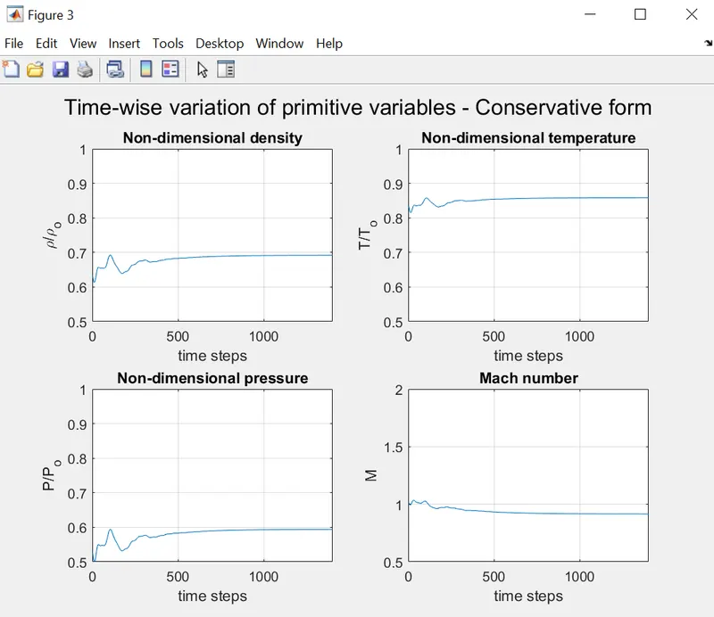
The first picture shows the primitive variables behavior at the nozzle throat, due to it is known the Mach number at this point is equal to 1 (sound speed), taking this value as stabilization reference. Analyzing the plot, the primitive variables achieve to get stabilization appoximately at 1000 time steps.

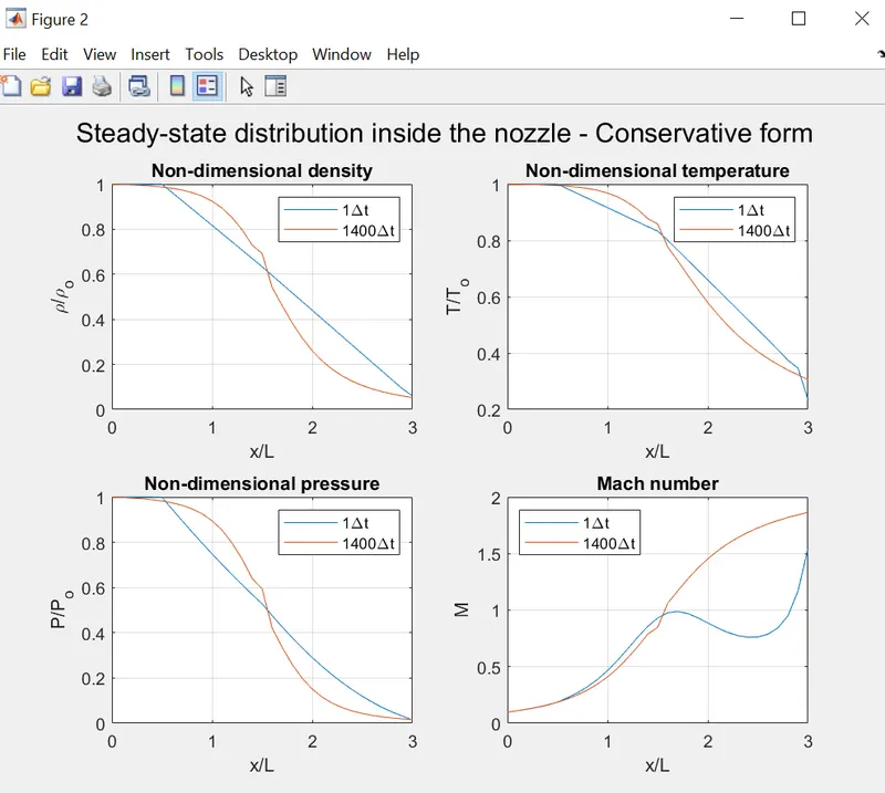
The stability previously assumpted can be clearly seen in the next picture,because of the function becomes less and less linear, fitting itself to a curvilineal function once the time step is equal to 1400.

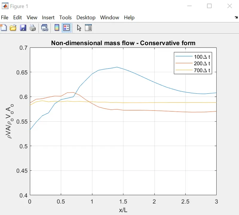
Finally, mass flow takes different behaviors until it reaches an approximated stabilization value, at 100 time steps there is a peak that once this time step increases, the peak decreases until becomes linear.

NON-CONSERVATIVE FORM

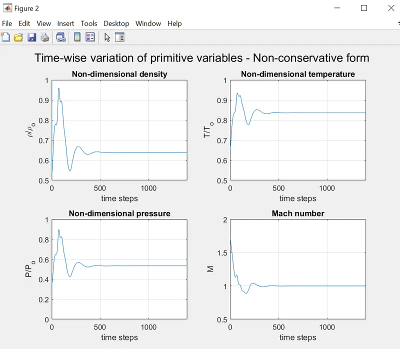
Regarding non-conservative form, analyzing the plot, the primitive variables achieve to get stabilization appoximately at 500 time steps, almost 500 time steps before than the conservative form.

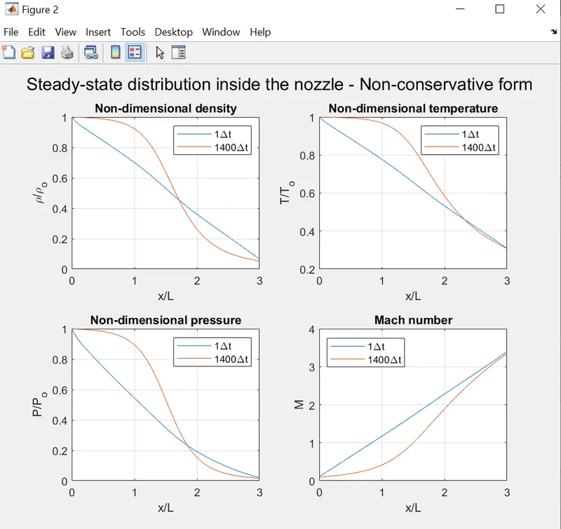
Likewise, the primitive variables at 1400 steps look more refined than the conservative form as it can be seen in the following plot picture.

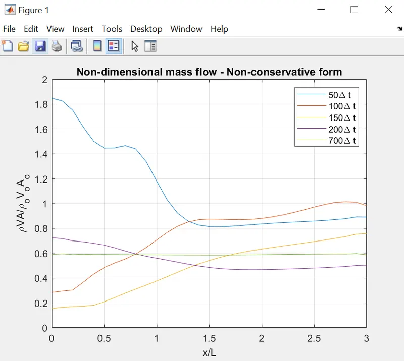
Mass flow behaves similar to the conservative form, but at 700 steps the mass flow is more linear than the conservative mass flow at 700 steps.

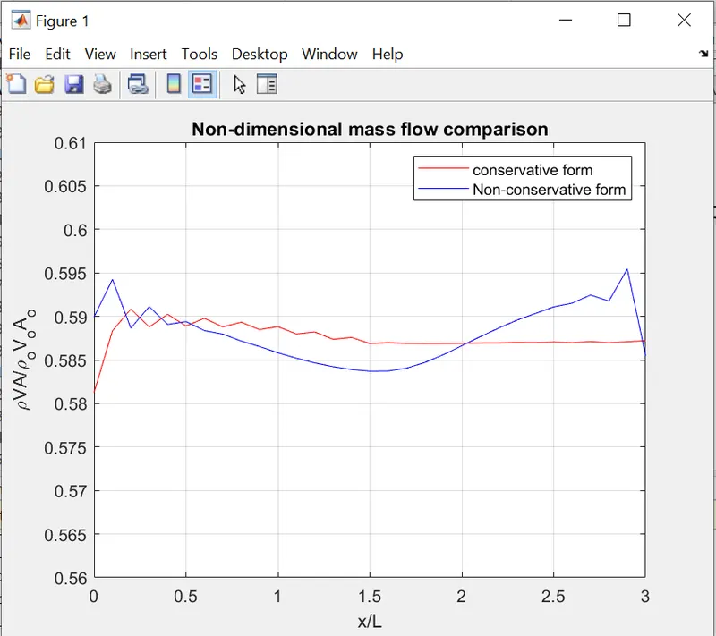
It can finally be determined the more efficient way to solve the 1D nozzle flow simulation is using non-conservative governing flow equations.

The picture shown above shows in a magnified scale the mass flow keeps more constant in conservative form than in non-conservative form; however, the real behavior is going to be the non-conservative form due to the area variation.

6. CONCLUSIONS

Governing flow equations are a keytool to get the an approximated mathematical behavior inside a convergent-divergent nozzle; this is so important because of the nozzle principle has allowed to perform different improvements on aerospace engineering, mechanical engineering, industrial engineering, nautical engineering and other different fields. Furthermore, Macormack tecnique becomes easier the way to iterate the PDE solutions but, in this case, in order to get an appropiate accuracy result, it is better to use non-conservative form equations than conservative equations.

That's it , thanks for reading

7. REFERENCES

https://airloads.net/Downloads/Textbooks/Computational-Fluid-Dynamics-the-Basics-With-Applications-Anderson-J-D.pdf

https://www.quora.com/In-CFD-what-is-conservative-and-non-conservative-form-of-Navier-Stokes-equation