Week 5.1 - Mid term project - Solving the steady and unsteady 2D heat conduction problem
Steady and Unsteady 2D Heat Conduction Solution Project
1. AIM
The following project is about the study of the steady and transient 2D heat conduction equation behavior, using different iteration solver methods. Solver methods require computational analysis to solve each value until the equation has the minimum error possible or stable, before the equation has been unstabilized due to the truncation error increasing. To do this, it will be used three mathematical methods which are Jacobi, Gauss-Seidel and Succssive Over-Relaxation method, methods commonly used in infinite elements and CFD fields. These three methods will be used in order to determine which one is the more efficient to reach the error range in less number of nodes for steady and transient 2D heat conduction implicit equation.
Transient equation will be solved using implicit and explicit function, so taking into account the values of the implicit function equation are unknown, this equation will be overwritted and as it was written above, this will be solved using iteration methods.
2. EQUATIONS
2.1. STEADY 2D HEAT CONDUCTION EQUATION
- PDE:
`(partial^2T)/(partialx^2)+(partial^2T)/(partialy^2)=0`
- Equation as Taylor approximation:
`(T(i-1,j)-2T(i,j)+T(i+1,j))/(Deltax^2)+(T(i,j-1)-2T(i,j)+T(i,j+1))/(Deltay^2)=0`
In the equation, the boundary values are known, however, center value must get an approximately accurate value to make the equation theory has been accomplished. The equation will be overwritten as:
`T(i,j)=(Deltay^2[T(i-1,j)+T(i+1,j)]+Deltax^2[T(i,j-1)+T(i,j+1)])/(2(Deltax^2+Deltay^2))`
2.2. TRANSIENT 2D HEAT CONDUCTION EQUATION
- PDE:
`alpha((partial^2T)/(partialx^2)+(partial^2T)/(partialy^2))=(partialT)/(partialt)`
- Equation as Taylor approximation - explicit form:
`alpha((T(i-1,j)-2T(i,j)+T(i+1,j))/(Deltax^2)+(T(i,j-1)-2T(i,j)+T(i,j+1))/(Deltay^2))^n=(DeltaT(i,j)^(n+1)-DeltaT(i,j)^n)/(Deltat)`
- Equation as Taylor approximation - implicit form:
`alpha((T(i-1,j)-2T(i,j)+T(i+1,j))/(Deltax^2)+(T(i,j-1)-2T(i,j)+T(i,j+1))/(Deltay^2))^(n+1)=(DeltaT(i,j)^(n+1)-DeltaT(i,j)^n)/(Deltat)`
Where n means the time loop and `alpha` the thermal diffusivity.
Similar to the steady function, the boundary and initial conditions are known, but in this case, it is necessary to know how the temperature change regarding the time change. To analyze it, it must be cheked each value into the space division. Therefore, the equation will look as:
`T(i,j)^(n+1)=T(i,j)^n+alpha(Deltat)/(Deltax^2)(T(i-1,j)-2T(i,j)+T(i+1,j))^n+alpha(Deltat)/(Deltay^2)(T(i,j-1)-2T(i,j)+T(i,j+1))^n`
In implicit function, the time loop will be analyzed taking the values in the same time loop value, so the equation is going to be:
`T(i,j)^(n+1)=T(i,j)^n+alpha(Deltat)/(Deltax^2)(T(i-1,j)-2T(i,j)+T(i+1,j))^(n+1)+alpha(Deltat)/(Deltay^2)(T(i,j-1)-2T(i,j)+T(i,j+1))^(n+1)`
3. OBJECTIVES
- Design a code to solve steady and transient 2D heat conducion equation, using different iteration solver methods.
- Plot the equation behavior for each method and type of heat conduction equation approximation.
- Determine the most efficient solver method, comparing the number of iterations taken in each method to reach the minimum error established.
4. PROJECT DEVELOPMENT
4.1. STEADY 2D HEAT CONDUCTION EQUATION SOLUTION:
Firstly, it must be defined the initial condition for steady function, so the accuracy deegre will be `Deltax^2`,and the approximation will be taken as centered difference approximation; furthermore, according to the project statements, the bottom temperature (Tb) and top temperature are(Tp):
Tb=900 K
Tt=600 K
Also,the left temperature (Tl) and right temperature (Tr) are:
Tl=400 K
Tr=800 K
All these temperatures are going to be located along the entire side assigned; the initial temperature into the space will be equal to 300K. The number of nodes of the whole square surface will be divided in a similiar portion as nx=ny=[Number of nodes], where nx is equal to the number of nodes on the x axis and ny is equal to the number of nodes on the y axis; the nodes division will be of 20 sections in order to see the behavior in a more accurate way. The length along the x and y axis will be 1 meter and the division between each node will be given by the length over the number of nodes.
Secondly, due to the temperature among the inner space seccion is unknown, it must be carried out an apporixomation of these values; Therefore, it will be used the following methods: 1) Jacobi Method ; 2) Gauss Seidel Method ; 3) SOR Method.
Jacobi method approahes the values taking the previous values calculated, until the absolute error between the old and new values is enough low. The steady equation is analyzed as:
`T(i,j)=(Deltay^2[Told(i-1,j)+Told(i+1,j)]+Deltax^2[Told(i,j-1)+Told(i,j+1)])/(2(Deltax^2+Deltay^2))`
Gauss Seidel Method approaches the values, taking in this case the current value that any term of the equation get at the moment. The equation will be written as:
`T(i,j)=(Deltay^2[T(i-1,j)+Told(i+1,j)]+Deltax^2[T(i,j-1)+Told(i,j+1)])/(2(Deltax^2+Deltay^2))`
The SOR (Succesive Over-relaxation Method)uses the value obtained by Gauss-Seidel or Jacobi method, and approaches the values as from the old values found as the new values obtained. SOR accelerates the convergence, however, the `omega` coefficient must not be neither less than zero nor greater than two. The equation should be written as:
`T(i,j)=omega*Told+(1-omega)*Trightarrow GS or Jacobi method`
For this solution, `omega` is going to take a value of 1,9.
Finally, having all of these parameters, it is going to be performed the analysis for steady 2D heat conduction equation and it will be plotted the equation behavior regarding each iteration. MATLAB code is attached below and, in the next link, it is shown how the equation is being fitted until the equation reaches an error value of `1*10^-4`. MATLAB code archive is also attached below as "Week_5.1_Mid_term_project_Solving_the_steady_and_unsteady_2D_heat_conduction_problem".
- Steady & Transient 2D Heat Conduction Equation Behavior at Different Iteration Solver Methods - Link:
- Steady 2D heat conduction equation solution - MATLAB code:
%Week 5.1.-Mid term project - Solving the steady and unsteady 2D heat conduction problem
%Diego Alejandro Cepeda Cuartas
%Aeronautical Engineer
%1. Steady state analysis & Transient State Analysis

%Solve the 2D heat conduction equation by using the point iterative techniques
%that were taught in the class. The Boundary conditions for the problem are
%as follows;

%Top Boundary = 600 K
%Bottom Boundary = 900 K
%Left Boundary = 400 K
%Right Boundary = 800 K

%You will implement the following methods for solving implicit equations.

%Jacobi
%Gauss-seidel
%Successive over-relaxation
%Your absolute error criteria is 1e-4

%Note: Make sure to use "INSERT CODE SAMPLE" option to paste the code here.
%Post screenshots of the plots and use the projects.skill-lync.com page to
%publish your findings.

%2. You will write code for both implicit and explicit schemes (This is for
%the transient analysis only)

%3. Compare the convergence rate [Number of iterations] of the steady state
%and transient [explicit and implicit] simulations and justify the numerics.

%CODE SOLUTION:
clear all
clc

%STEP 1: Defining the accuracy deegre of the equation.
%The accuracy deegre will be DX^2,and the approximation will be taken as
%centered difference approximation.

%STEP 2: Entering the initial conditions.
%According to the project statements, the bottom temperature (Tb) and top
%temperature are(Tp):
Tb=900 %K
Tt=600 %K

%Furthermore,the left temperature (Tl) and right temperatur (Tr) are:
Tl=400 %K
Tr=800 %K

%The number of nodes of the whole square surface will be divided in a
%similiar portion as nx=ny=[Number of nodes], where nx is equal to the
%number of nodes on the x axis and ny is equal to the number of nodes on
%the y axis. The length along the x and y axis will be 1 meter and the
%division between each node will be given by the length over the number of
%nodes.

L=1 % meter in each side

nx=20 %number of nodes in x
ny=nx %number of nodes in y
x=linspace(0,1,nx)
y=linspace(0,1,ny)

dx=L/nx %sloop among the Lx axis
dy=L/ny %Sloop among the Ly axis

%The initial temperature conditions described above on the space delimited
%is distributed as:

T=ones(nx,ny)*300 %K according to the challenge rules

T(:,1)=Tl %Temperature at the left side
T(1,:)=Tb %Temperature at the bottom side
T(:,end)=Tr %Temperature at the right side
T(end,:)=Tt %Temperature at the top side

%Furthermore, the average values in the corner boundaries:

T(end,end)=700 %K
T(1,1)=650 %K
T(1,end)=850 %K
T(end,1)=500 %K
Told=T
%STEP 3: Solving steady 2D heat conduction behavior
%Steady 2D heat conduction behavior equation is:
%(dT/dx)^2+(dT/dy)^2=0

%Using taylor series aproximation equations, the equation will be:
%[(T(i-1,j)-2*T(i,j)+T(i+1,j))/(dx^2)]+[(T(i,j-1)-2*T(i,j)+T(i,j+1))/(dy^2)]=0

%Solving the equation, the equation will fit as:
%T(i,j)=((dy^2)[T(i-1,j)+T(i+1,j)]+(dx^2)[T(i,j-1)+T(i,j+1)])/2[(dx^2)+(dy^2)]

%Due to the temperature among the inner space seccion is unknown, it must
%be carried out an apporixomation of these values; Therefore, it will be
%used the following methods: 1) Jacobi Method ; 2) Gauss Seidel Method ;
% 3) SOR Method.

method=input("Enter the method you need to use: 1) Jacobi, 2)Gauss-Seidel, 3) SOR:  ")

%The permissible error is 1e-4:
error=9e9;
tol=1e-4;

%Finally, having all of these parameters, it is going to be performed the
%analysis for steady 2D heat conduction equation and then, it will be
%analyzed the equation once this one is in unsteady condition:

if method==1
    display('Jacobi Method')
    j_iter=1
    while (error>tol)
        for i=2:nx-1
            for j=2:ny-1
                term1=(dy^2)*(Told(i-1,j)+Told(i+1,j));
                term2=(dx^2)*(Told(i,j-1)+Told(i,j+1));
                T(i,j)=(term1+term2)/(2*((dx^2)+(dy^2)));
            end
        C=contourf(x,y,T);
        clabel(C)
        colormap(jet)
        colorbar
        xlabel("X axis")
        ylabel("Y axis")
        title('Jacobi Method - Iteration number=',j_iter)
        pause(0.001)
        end
        error=max(max(abs(Told-T)))
        Told=T;
        j_iter=j_iter+1
    end


elseif method==2
    display('GS Method')
        GS_iter=1
    while (error>tol)
        for i=2:nx-1
            for j=2:ny-1
                term1=(dy^2)*(T(i-1,j)+Told(i+1,j));
                term2=(dx^2)*(T(i,j-1)+Told(i,j+1));
                T(i,j)=(term1+term2)/(2*((dx^2)+(dy^2)));
            end
        C=contourf(x,y,T);
        clabel(C)
        colormap(jet)
        colorbar
        xlabel("X axis")
        ylabel("Y axis")
        title('Gauss-Seidel Method - Iteration number=',GS_iter)
        pause(0.001)
        end
        error=max(max(abs(Told-T)))
        Told=T;
        GS_iter=GS_iter+1
    end


elseif method==3
    display('SOR Method')
    omega=1.9
    SOR_iter=1
    while (error>tol)
        for i=2:nx-1
            for j=2:ny-1
                term1=(dy^2)*(T(i-1,j)+Told(i+1,j));
                term2=(dx^2)*(T(i,j-1)+Told(i,j+1));
                Tgs=(term1+term2)/(2*((dx^2)+(dy^2)))
                T(i,j)=(Told(i,j)*(1-omega))+(omega*Tgs);
            end
        C=contourf(x,y,T);
        clabel(C)
        colormap(jet)
        colorbar
        xlabel("X axis")
        ylabel("Y axis")
        title('SOR Method - Iteration number=',SOR_iter)
        pause(0.001)
        end
        error=max(max(abs(Told-T)))
        Told=T;
        SOR_iter=SOR_iter+1
    end
end

% Now, the unsteady 2D heat conduction behavior is going to depend of the
% initial conditions regarding the change of time, to perform this analysis
%the new code will take the Jacobi, Gauss-Seidel and SOR iteration methods,
%and it will be updated the temperature values in each time loop. The
%equation in this case is:

%T(i,j)= T_previous(i,j)+K1[Told(i-1,j)-2Told(i,j)-Told(i+1,j)]+K2[Told(i,j-1)-2Told(i,j)-Told(i,j+1)]

%Where:

%K1=alpha*(dt/dx^2)
%K2=alpha*(dt/dy^2)

%Those two parameters must be less than 0.5, otherwise, the equation is
%going to be unstable. Told will be the temperature conditions that will be
%updated before updating the temperature in an instance of time.

% Transient 2D heat conduction sotucion code is attached on the MATLAB
% sheet "5.1.Transient_Function".
4.2. TRANSIENT 2D HEAT CONDUCTION EQUATION SOLUTION:
Firstly, aking into account the initial conditions are going to be equals to the conditions exposed in the steady function, except the node division that will be equal to 15, it will only explain the in this part the implicit and explicit solution.
Now, to solve transient 2D heat conduction equation, explicit solution only takes the old values calculated at the previous time loop , then the equation in this case will be:
`T(i,j)^(n+1)=T(i,j)^n+alpha(Deltat)/(Deltax^2)(T(i-1,j)-2T(i,j)+T(i+1,j))^n+alpha(Deltat)/(Deltay^2)(T(i,j-1)-2T(i,j)+T(i,j+1))^n`
However, implicit function takes the values at the same time loop in what the time is, due to that, almost all the values are unknown except the previous value that accompanied the time term, that is equal to the previous values calculated. Furthermore, Courant number plays an important role in this equation because of the sum between the x term relation and y term relation must be less or equal than 0,5. Therefore, the thermal difussivity has to take a value which keeps the x and y relation among the Courant theorem range.
`alpha(Deltat)/(Deltax^2)+alpha(Deltat)/(Deltay^2)<=0,5`
So, the thermal diffusivity is going to be equal to `alpha=1.5` and the time loop will take 1500 loops. In this part, `alpha(Deltat)/(Deltax^2)` will be called as K1 and `alpha(Deltat)/(Deltay^2)`is going to be called as K2. the number of nodes as in x as in y are similar, so the K1 and K2 ratio will be equal too. In this case K1=0,0338 and K2=0,0338.
The initial equation for implicit function will stay as:
`T(i,j)^(n+1)=T(i,j)^n+K1(T(i-1,j)-2T(i,j)+T(i+1,j))^(n+1)+K2(T(i,j-1)-2T(i,j)+T(i,j+1))^(n+1)`
But, arranging the similar terms and solving the equation, the implicit function equation will be written as:
`T(i,j)^(n+1)=(1)/(1+2K1+2K2)*[T(i,j)^n+K1(T(i-1,j)-2T(i,j)+T(i+1,j))^(n+1)+K2(T(i,j-1)-2T(i,j)+T(i,j+1))^(n+1)]`
Finally, the two equations can be solved using an algorith code, which as similar as the steady function, was written on MATLAB and attached below. In the link attached above, it can be check out the equation behavior for each type of solution carried out. MATLAB code archive is also attached below as "5.1.Transient_Function".
Transient 2D heat conduction equation solution - MATLAB code:
%CODE SOLUTION:
clear all
close all
clc

%STEP 1: Defining the accuracy deegre of the equation.
%Because of it have only got the values from top, bottom, right
%and left sides of the center point, the accuracy deegre will be DX^2,and
%the approximation will be taken as centered difference approximation.

%STEP 2: Entering the initial conditions.
%According to the project statements, the bottom temperature (Tb) and top
%temperature are(Tp):
Tb=900 %K
Tt=600 %K

%Furthermore,the left temperature (Tl) and right temperatur (Tr) are:
Tl=400 %K
Tr=800 %K

%The number of nodes of the whole square surface will be divided in a
%similiar portion as nx=ny=[Number of nodes], where nx is equal to the
%number of nodes on the x axis and ny is equal to the number of nodes on
%the y axis. The length along the x and y axis will be 1 meter and the
%division between each node will be given by the length over the number of
%nodes.

L=1 % meter in each side

nx=15 %number of nodes in x
ny=nx %number of nodes in y
x=linspace(0,1,nx)
y=linspace(0,1,ny)

dx=L/nx %sloop among the Lx axis
dy=L/ny %Sloop among the Ly axis

%The initial temperature conditions described above on the space delimited
%is distributed as:

T=ones(nx,ny)*300 %K according to the challenge rules

T(:,1)=Tl %Temperature at the left side
T(1,:)=Tb %Temperature at the bottom side
T(:,end)=Tr %Temperature at the right side
T(end,:)=Tt %Temperature at the top side

%Furthermore, the average values in the corner boundaries:

T(end,end)=700 %K
T(1,1)=650 %K
T(1,end)=850 %K
T(end,1)=500 %K
Told=T

% Now, the unsteady 2D heat conduction behavior is going to depend of the
% initial conditions regarding the change of time, to perform this analysis
%the new code will take the Jacobi, Gauss-Seidel and SOR iteration methods,
%and it will be updated the temperature values in each time loop. The
%equation in this case is:

%T(i,j)= T_previous(i,j)+K1[T_previous(i-1,j)-2T_previous(i,j)-T_previous(i+1,j)]+K2[T_previous(i,j-1)-2T_previous(i,j)-T_previous(i,j+1)]

%Where:

%K1=alpha*(dt/dx^2)
%K2=alpha*(dt/dy^2)

%Those two parameters must be less than 0.5, otherwise, the equation is
%going to be unstable. Told will be the temperature conditions that will be
%updated before updating the temperature in an instance of time.
%The implicit function is the function described above, but, for explicit
%function, the equation changes due to the time value is evaluated at the
%moment of the neighbor values are in the same time loop. To find all these
%values, it is used the iteration method solvers named before. The explicit
%equation will be:

%T(i,j)=(1/1+(2*K1)+(2*K2))*(T_previous(i,j)+K1*(Told(j-1,k)+Told(j+1,k))+k2*(Told(j,k-1)+Told(j,k+1)))

T_previous=T

dt=1/10000; %Time loop
alpha=1.5 %diffusivity coefficient

%CFL:
K1=alpha*(dt/dx^2);%CFLx
K2=alpha*(dt/dy^2);%CFLy

 tol=1e-4

type=input('Choose 1)Explicit, 2)Implicit:')

if type==1
    %  EXPLICIT FUNCTION
    error=1e2
    explicit=0
    %Time loop
    while error>tol
            for j=2:nx-1
                for k=2:ny-1
                    T(j,k)=(T_previous(j,k))+(K1*(T_previous(j-1,k)-2*T_previous(j,k)+T_previous(j+1,k)))+(K2*(T_previous(j,k-1)-2*T_previous(j,k)+T_previous(j,k+1)));
                end
            end
            error=max(max(abs(T-T_previous)));
            T_previous=T;
            explicit=explicit+1
            C=contourf(x,y,T);
            clabel(C)
            colormap(jet)
            colorbar
            xlabel("X axis")
            ylabel("Y axis")
            title('Explicit form - Time=',explicit)
            pause(0.0001)
        end

    %IMPLICIT FUNCTION
elseif type==2
    method2=input('Now, enter the method you need to use for analyzing the rate of temperature change regarding the time: 1) Jacobi, 2)Gauss-Seidel, 3) SOR: ')

        %Time loop
    if method2==1
        display('Jacobi Method')
        jacobi=0;
        %Time loop
        for i=1:1500
            error_t=1e2;

            %Space term
            while (error_t>tol)
                for j=2:nx-1
                    for k=2:ny-1
                        term1=(1+(2*K1)+(2*K2))^-1;
                        term2=K1*term1;
                        term3=K2*term1;
                        T(j,k)=(term1*T_previous(j,k))+(term2*(Told(j-1,k)+Told(j+1,k)))+(term3*(Told(j,k-1)+Told(j,k+1)))
                    end
                end
                jacobi=jacobi+1;
                error_t=max(max(abs(Told-T)));
                Told=T;
            end
            T_previous=T
            C=contourf(x,y,T);
            clabel(C)
            colormap(jet)
            colorbar
            xlabel("X axis")
            ylabel("Y axis")
            title('Implicit form by Jacobi - Time=',i)
            pause(0.0001)
        end
    elseif method2==2
        display('Gauss-Seidel Method')
        GS=0;
        %Time loop
        for i=1:1500
            error_t=1e2;

            %Space term
            while (error_t>tol)
                for j=2:nx-1
                    for k=2:ny-1
                        term1=(1+(2*K1)+(2*K2))^-1;
                        term2=K1*term1;
                        term3=K2*term1;
                        T(j,k)=(term1*T_previous(j,k))+(term2*(T(j-1,k)+Told(j+1,k)))+(term3*(T(j,k-1)+Told(j,k+1)))
                    end
                end
                GS=GS+1;
                error_t=max(max(abs(Told-T)));
                Told=T;
            end
            T_previous=T
            C=contourf(x,y,T);
            clabel(C)
            colormap(jet)
            colorbar
            xlabel("X axis")
            ylabel("Y axis")
            title('Implicit form by Gauss-Seidel - Time=',i)
            pause(0.0001)
        end
    elseif method2==3
        display('SOR Method')
        omega=1.02
        SOR=0;
        %Time loop
        for i=1:1500
            error_t=1e2;

            %Space term
            while (error_t>tol)
                for j=2:nx-1
                    for k=2:ny-1
                        term1=(1+(2*K1)+(2*K2))^-1;
                        term2=K1*term1;
                        term3=K2*term1;
                        Tgs(j,k)=(term1*T_previous(j,k))+(term2*(T(j-1,k)+Told(j+1,k)))+(term3*(T(j,k-1)+Told(j,k+1)));
                        T(j,k)=Told(j,k)*(1-omega)+(omega*Tgs(j,k));
                    end
                end
                SOR=SOR+1;
                error_t=max(max(abs(Told-T)));
                Told=T;
            end
            T_previous=T
            C=contourf(x,y,T);
            clabel(C)
            colormap(jet)
            colorbar
            xlabel("X axis")
            ylabel("Y axis")
            title('Implicit form by SOR - Time=',i)
            pause(0.0001)
        end
    end
end
5. RESULTS
5.1. Steady 2D heat conduction equation solution
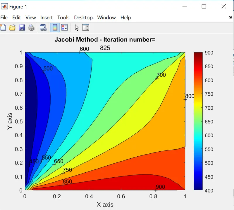
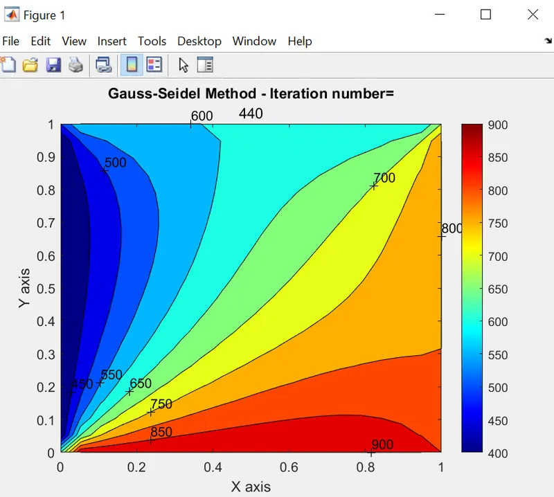
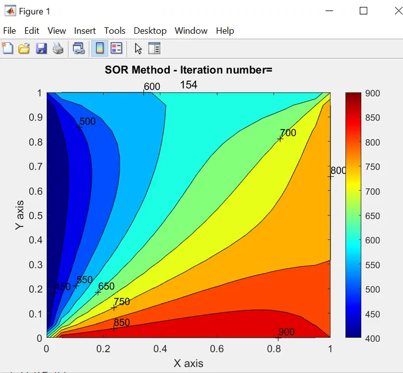
Comparing the iterations taken for each method, it can be seen the SOR method reaches the convergence in a less number of iterations than Jacobi and Gauss Seidel methods. However this is only possible if the `omega` coefficient is correctly selected. `omega` was taken as 1,9, but if the value would have been less than 1, the converge would have delayed even more than Gauss Seidel and Jacobi method.
In the pictures below are shown the convergence result in different solver method and the number of iterations taken by each one.
- Jacobi: 825
- Gauss Seidel: 440
- SOR: 154 at `omega=`1.9
5.2. Transient 2D heat conduction equation solution
5.2.1. Explicit time
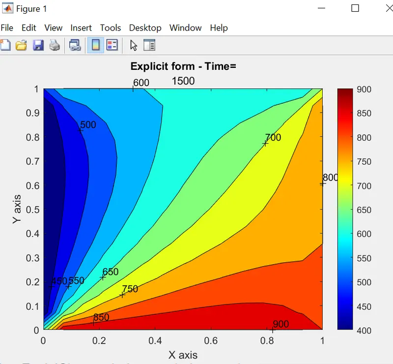
Explicit function has been defined in order to get the time loop that will converge with an error less or equal to `1*10^-4`. The number of iterations is even greater than the Jacobi method at steady condition, because of the CFL number for x and y taken in this section, delays the incresing of the temperature. The picture below shows the explicit form plot result.
- Explicit function: 2928 time loops
5.2.2. Implicit time
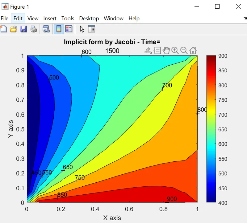
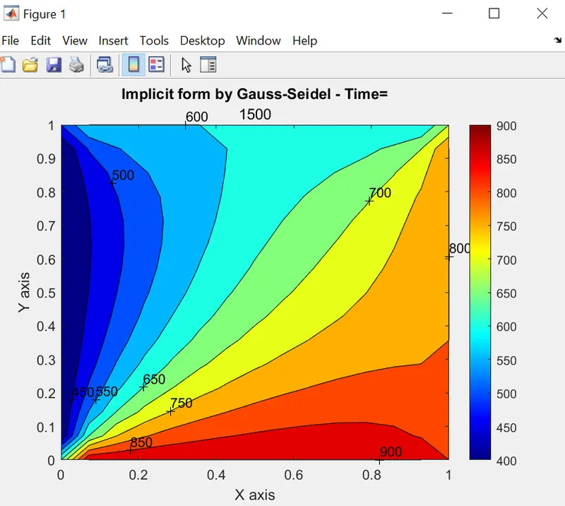
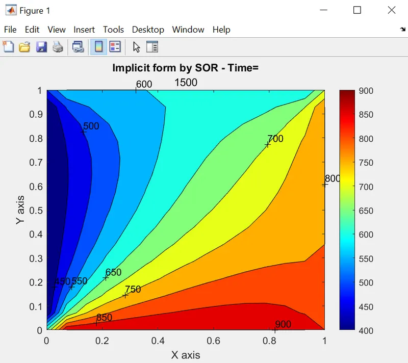
Implicit function interations are even more extend than explicit function, due to almost all its terms are unknown, therefore, it is firstly necessary to find the better values that can fit with the real function behavior and checking the following plots, Jacobi takes more iterations than Gauss Seidel and Gauss also take more iterations than SOR method, such as Steady condition analysis. However, if the `omega`coefficient is greater than 1,5, the function will take too much iterations to reach the convergence, it was found the function will converge at 120403 iterations when `omega`coefficient is 1,9, but at 1,02 `omega`coefficient, the function will converge at 5694 iterations, being different than the `omega` value in steady condition.
- Jacobi: 7334
- Gauss Seidel: 6234
- SOR: 5694 at `omega=`1.02; 120403 at `omega=`1.9
6. CONCLUSIONS
Steady function take less iterations to reach the convergence in comparison with transient function, CFL number triggers a convergence delay due to the low number value; however, this value must be taken such that the function achieves the convergence and keeps also stable.
Implicit transient function reaches the convergence quicker when SOR method iteration is used, due to the SOR method approximate the Jacobi and Gauss Seidel values obtained along with the previous value obtained. SOR method differs in both cases because of the equation gain more terms in transient conditions, that could mean if the function adds more terms, the `omega`coefficient should decrease in order to obtain the convergence in a low number of iterations.
Iteration solver methods have different field uses thanks to the quickly way to solve complex equations; some of these fields are CFD (Computational Fluid Dynamics), FEM (Finite Element Methods) and even in economic fields.
That's it, thanks for reading. Watch the project video here: https://youtu.be/N65VdF3dlic
7. REFERENCES
https://mathworld.wolfram.com/SuccessiveOverrelaxationMethod.html
https://functionbay.com/en/faq/single/263/differences-implicit-method-explicit-method