Week 5 - Turbulence modelling challenge
Turbulence Modeling Around a Golf Ball
AIM
The following project will simulate the flow behavior of a golf ball dived into an airflow field. It will first explain the turbulence solver methods currently known, and the best method for carrying out the simulation; then, the geometry given will be prepared and meshed according to Kolmogorov's scale length assumption, taken from the turbulence model selected; finally, the golf ball behavior will be analyzed and the wake regions obtained on the simulation will be explained.
Kolmogorov's scale is a method to identify the primitive parameters of an eddy that was created over an object by the viscous effects of the fluid; These eddies can be predicted by using the turbulence model solvers that will be explained later, and these solvers also takes the assumptions taken from the Kolmogorov's equation. Equations are obtained by taking the dissipation rate of the energy to determine the increase of the eddy; these equations are:
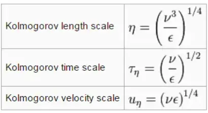
Image taken from: https://www.nuclear-power.com/nuclear-engineering/fluid-dynamics/turbulent-flow/kolmogorov-microscales-2/
Where `epsilon` is the dissipation rate of the enery and `vartheta`is the kinematic viscosity of the fluid. Then, Kolmogorov's equations can be rearranged and the following Kolmogorov's ratio takes place:
`L/eta=((U*L)/vartheta)^(3/4)=Re^(3/4)`
And this equation represents a great problem nowadays, because if the Reynolds number is higher than `10^6`, the simulation should take `10^14` grid points, which is impossible to do for the existing computers.
OBJECTIVES
Determine the best turbulence modeling solver, either DNS, RANS, or LES, to carry out the flow simulation over the golf ball provided by the challenge statements.
Use the Kolmogorov scale together with the `Y+` assumptions to perform the meshing over the golf ball.
Analyze the flow behavior by considering the ball is completely smooth at the bottom and there are some concave surfaces around the entire top section.
ENGINEERING DEVELOPMENT
To carry out the flow simulation over the golf ball, it will be first analyzed the best fluid dynamics modeling the simulation should use; there are three common types of fluid dynamics models named as DNS (Direct Numerical Simulation), LES (Large Eddies Simulation), and RANS (Reynolds Average Navier-Stokes).
DNS (Direct Numerical Simulation) is commonly known for its high computational cost and its highly accurate results; DNS is used in simulations where the near-wall separated flow must be explained or things that need to be highly accurate, however, this method is not feasible in comparison with LES and RANS methods, which are obtained by DNS.
LES (Large Eddies Simulation) is used for solving large eddy behavior because the LES model takes the fact that the energy travels from the large turbulence scales to the smaller ones. Thus, LES is based on solving the large eddies generated by the fluid disturbing and the small eddies using a modeling known as SGS modeling; This turbulence modeling should be more accurate than RANS, nevertheless, at high Reynolds numbers the predictions are better in RANS, due to the small eddies dissipation present on the near wall takes place and it is not taken into account by the LES model. It is then used as a variant of LES model known as LES/RANS, which combines the LES model and the RANS model altogether.
RANS (Reynolds Average Navier-Stokes) is the turbulence model most used in the industry because the computational cost is less than the other two models. RANS is not too accurate but it can be used to approximate the flow behavior in any component just by using a good wall treatment without the need of a kind of supercomputer, in comparison with DNS and LES models. These comparisons can be checked in the following table:
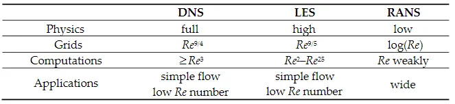
Table taken from: https://www.researchgate.net/publication/354225789_Improving_the_Energy_Efficiency_of_Buildings_Based_on_Fluid_Dynamics_Models_A_Critical_Review
The grid range is obtained by Kolmogorov's scale, and if the grid is divided according to each grid equation obtained, it will be easy to know the DNS model will have too small elements and the RANS will have the biggest elements if a simulation was carried out with each model. the DNS model would take too much time to get an accurate result and even the new computers do not have enough capability to reach a result faster than RANS. Thus, Kolmogorov's scale also shows that the DNS model is not a feasible method to resolve turbulence models yet; Even LES model is too heavy to simulate with this one.
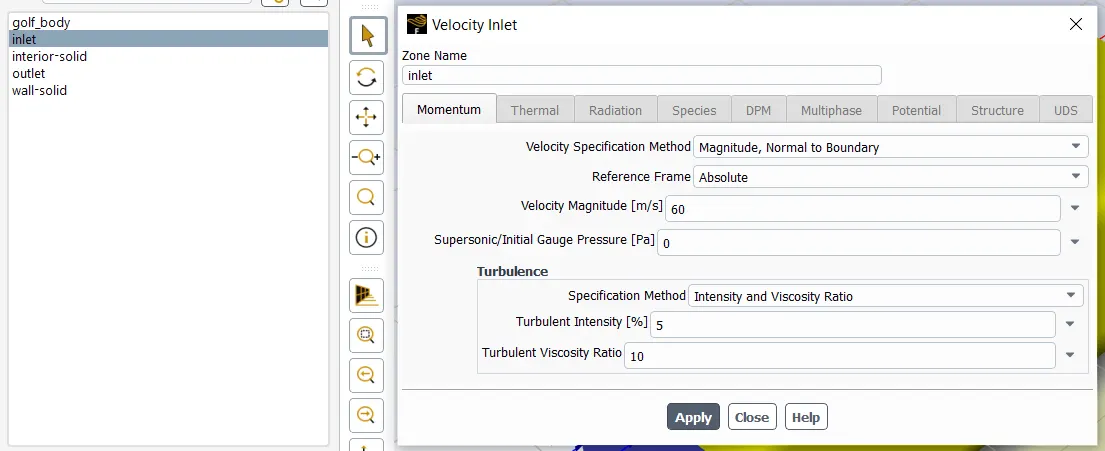
Now, according to the challenge statements, the speed at which the golf ball is traveling is equal to 60 `m/s`, and checking the golf ball diameter of the file provided by the challenge, the sample has a diameter of `6.3 mm`. Considering these parameters and assuming the flow is airflow at standard conditions, the Reynolds number obtained will be equal to `25.9*10^3`.
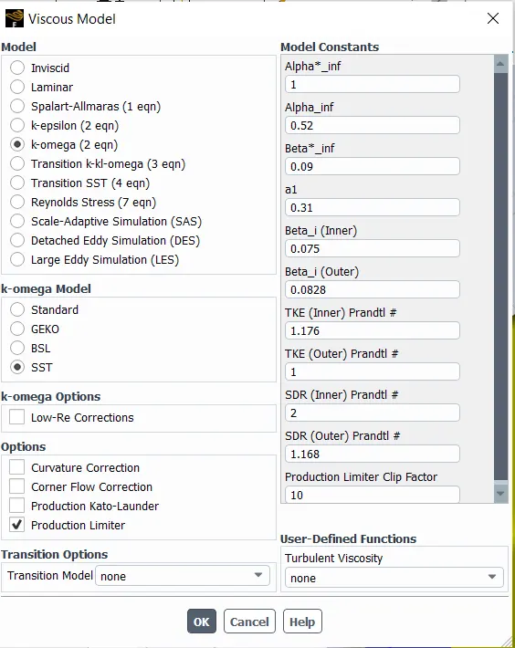
In this case, the RANS model is taken to perform the simulation, and the RANS turbulence model solver chosen is `k-omega` SST model, thanks to this turbulence model solver can simulate the separated flow in a highly accurate way.
To start preparing the geometry given by the challenge, it is calculated the ideal element size that the cells should measure to get an accurate result. according to the table shown above, the RANS equation will be given as:
`l_c/eta=log(Re)`
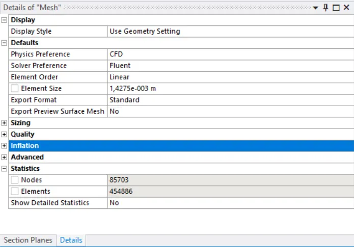
Where `l_c` is the eddy length and `eta` the Kolmogorov's length scale. Then, the ideal grid size should be equal to 0.00023m. Taking this assumption, the program licenses will not allow to perform the simulation, because the element size will exced the limit range. Then, the mesh is generated over the object with an element size of 0.00142 m, as is shown in the following picture.
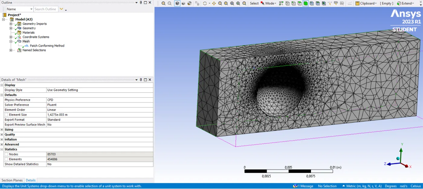
By default, the program makes the cells near the golf ball walls to have a size smaller than the cells far from the golf ball geometry.
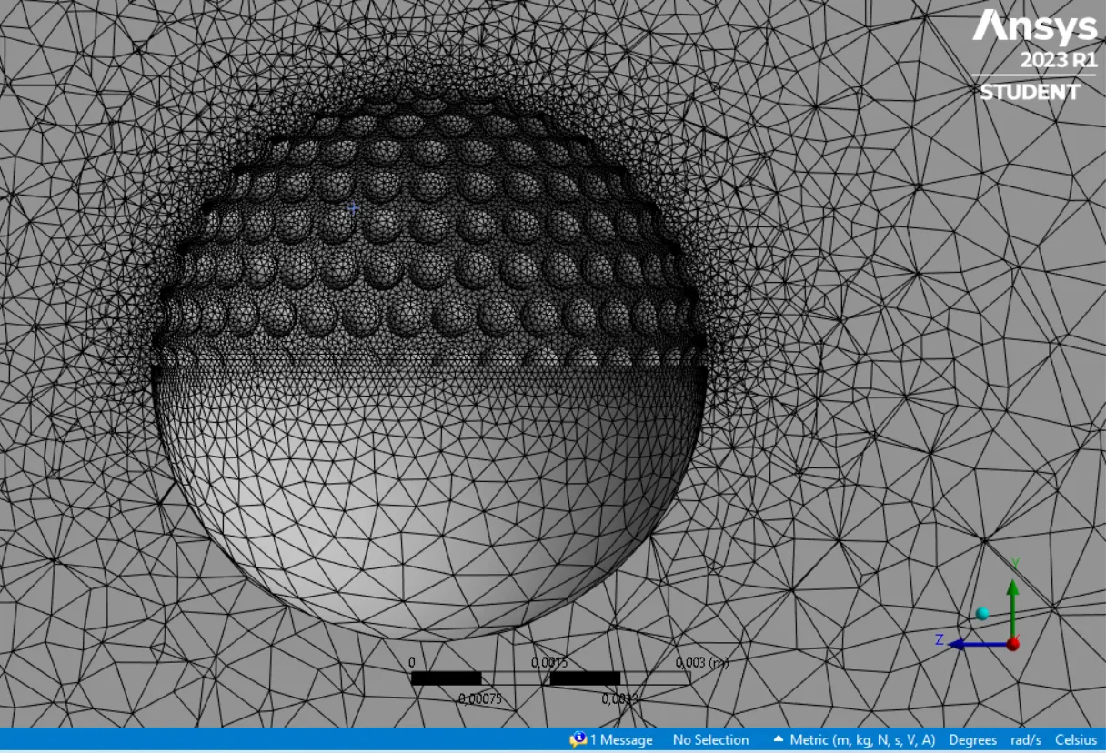
Using the element size value assumed, the number of elements is in the student license limits.
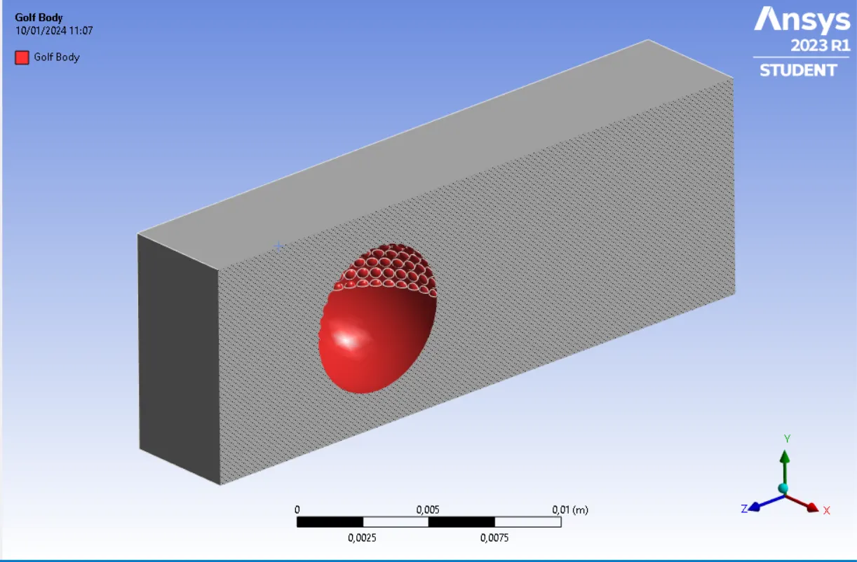
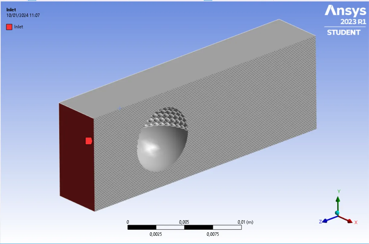
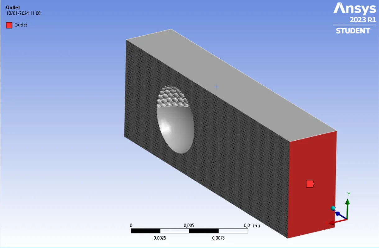
Another important thing is to define the components that the geometry has, being the golf ball surface, the inlet, the outlet, and the free-stream volume; only the free-stream volume is not defined because ANSYS takes it by default, once the geometry meshed is taken to the solver section.
- Golf ball surface
- Inlet
- Outlet
The next step is to simulate the flow over the golf ball; as the pictures previously attached show, the golf ball has a smooth circular shape at the bottom and a surface with little concave surfaces at the top. This geometry was made in this way to analyze the flow behavior around each type of surface, and determine the wake regions. So, the general parameters must be set as is shown in the next image.
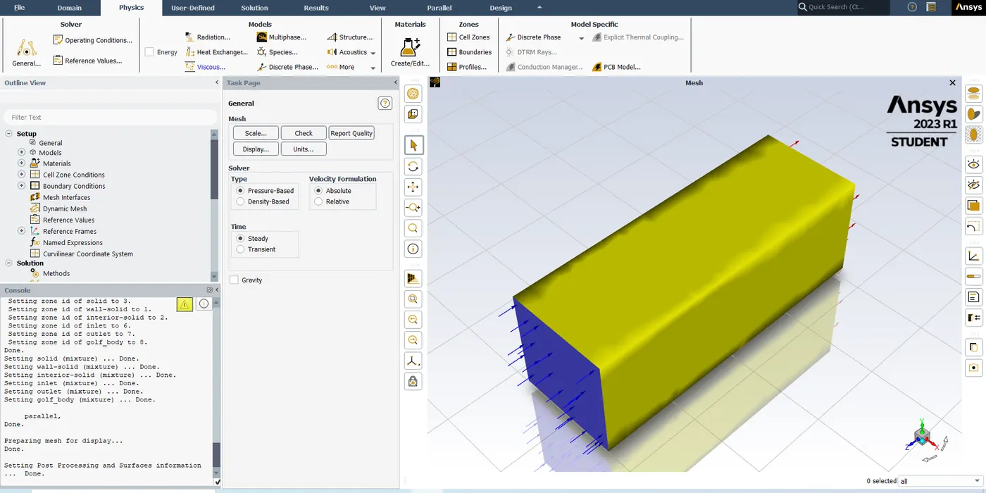
Likewise, `k-omega` SST model is put into the viscous model. All the constants remain as the program throw them by default.
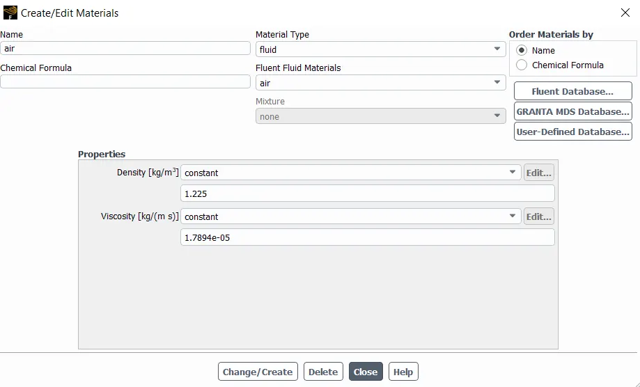
The flow will be airflow at standard conditions as it was described above.
At the inlet section, the velocity is entered and the other sections remain as the program set them by default.
Finally, the simulation is run out at 250 iterations; it can also be recorded the convergence reaching by taking snapshots of the velocity field result in each iteration.
RESULTS
The streamlines will get the movement shown in the following picture.
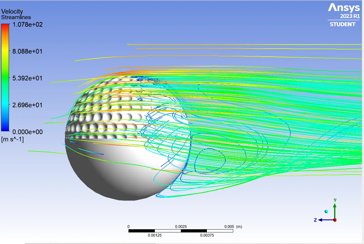
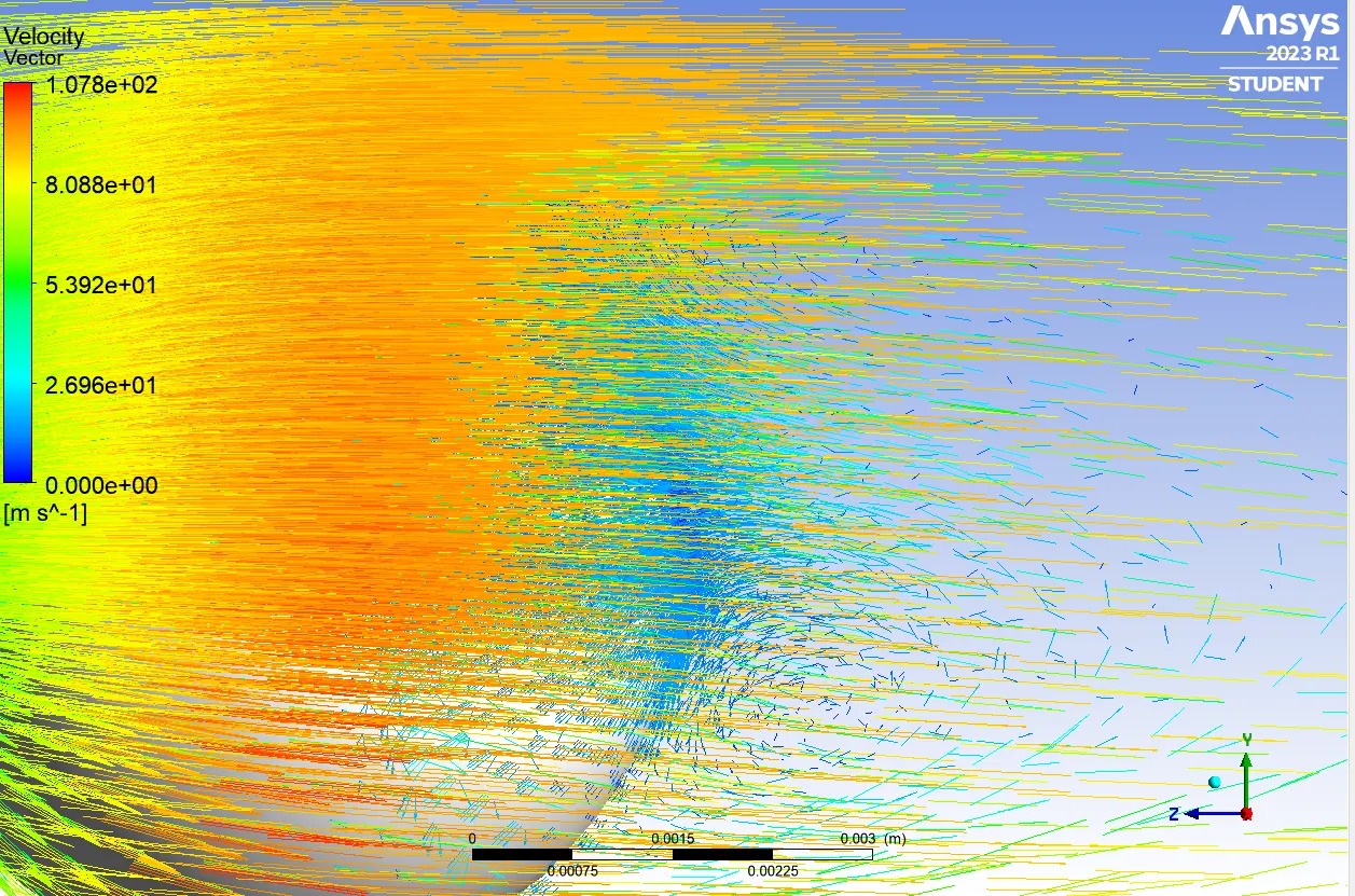
In the same way, the flow particles will trigger eddies at the back of the golf ball, generating also wake regions and increasing the drag force as is shown in the image below.
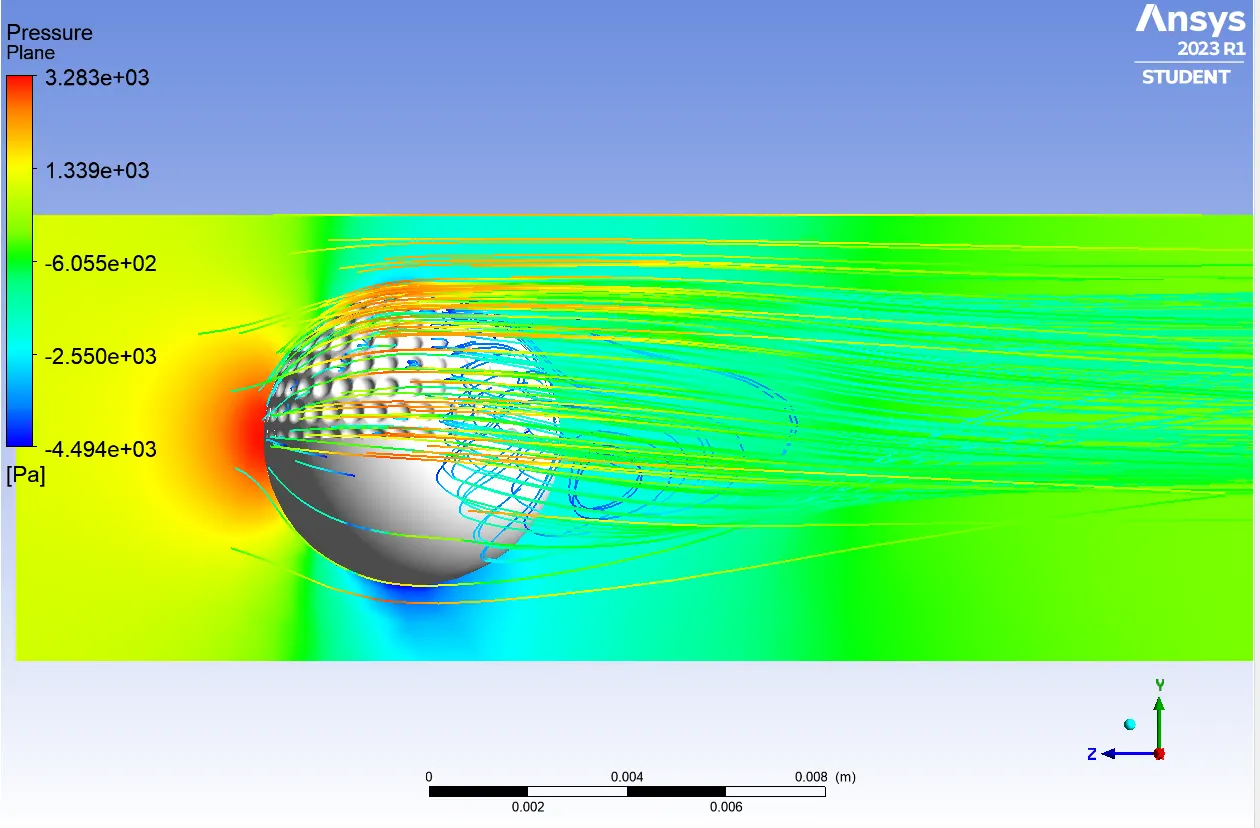
Then, looking at the pressure field, it can be seen the weakest region occurs at the bottom of the golf ball, as it was expected.
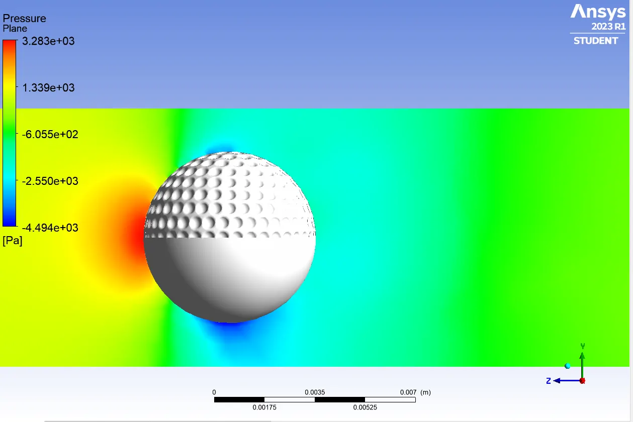
The main reason for this behavior is that the flow separation is reached at a large distance on smooth surfaces or even on surfaces that have convex sections over them. This flow separation gains too much energy, making the object loses pressure, and the stagnation pressure commonly generated in front of the object becomes a pressure drag over the object, while the concave sections over the top surface trigger that the pressure and velocity vary in each concave section, without allowing the flow separation occurs with high energy. The image below shows the streamlines in comparison with the velocity field plane.
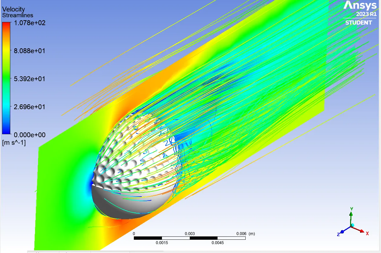
Similar to the previous image, the streamlines are compared with the pressure field plane, and it is deduced that the large eddy generated at the bottom of the back, can be taken as a section where the wake region is mainly present.
CONCLUSIONS
RANS model can get an expected result about the turbulence movement of the flow around a body, however, DNS and LES would get better results than RANS because their cells are small enough that each flow particle can be tracked in an element with less volume. To achieve the use of these methods, computers should have a better quantity capability which is currently not easy to reach; only some computers can use these methods, but those computers are too expensive.
Wake regions can be neglected by making the object's surface vary the pressure and velocity gradients, making the velocity profile not trigger large eddies due to the quick flow separation. This analysis is carried out in other components or machines, to mitigate the drag coefficient increase generated by the adverse pressure gradient.
According to the simulation, the ball will get an anticlockwise moment, because the drag force is greater at the bottom than at the top of the golf ball. Furthermore, the ball will drop so fast due to the pressure gradient is higher at the top section.
REFERENCES
https://www.simscale.com/docs/tutorials/compressible-cfd-simulation-golf-ball/