Week 8- Moving zones approach in Fluent

Moving Zones Approach in Fluent

AIM

The moving zones approach is a well-known method that involves the flow behavior simulation of components whose domain or parts from the domain are in movement like impellers, turbomachines, pumps, etc. ANSYS Fluent provides three approaches known as:

• the multiple reference frame (MRF) model
• the mixing plane model
• the sliding mesh model

The first two models assume that the flow field is steady; these two cases are acceptable in cases where the stator-rotor has a weak interaction with the flow and, the sliding mesh assumes that the flow is unsteady; this method is acceptable in cases where the rotor-stator interaction with the field strong.

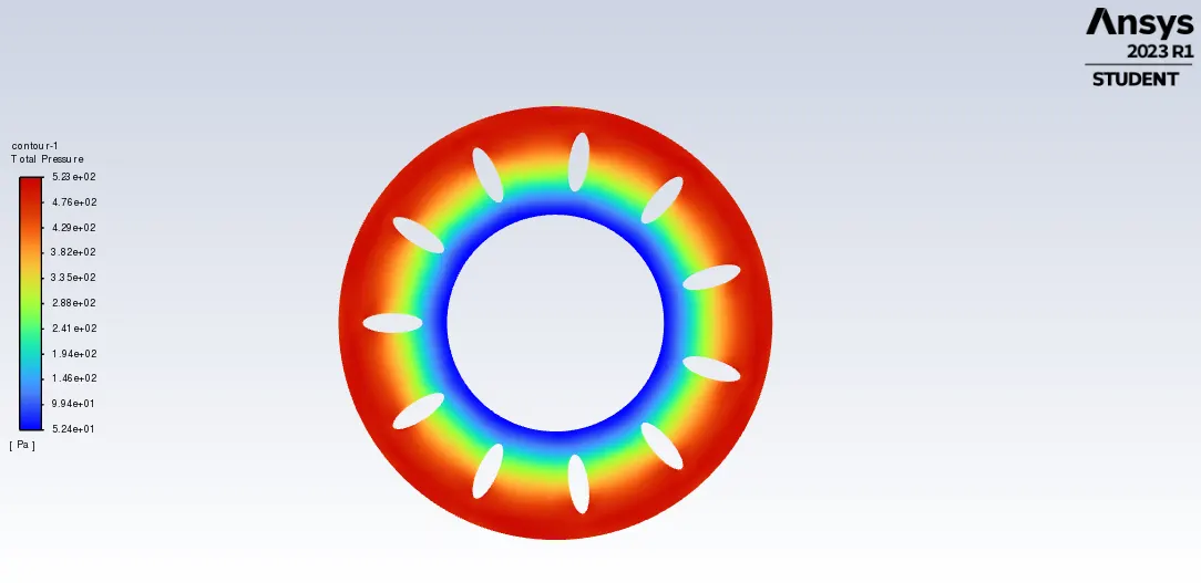
In this project, it will simulate a configuration of airfoils that are going to rotate inside a circular domain. It will use the mesh file provided by the project statements, and the steps to carry out the simulation will be performed and shown. Finally, the velocity profile and pressure profile will be plotted.

In addition, to carry out this simulation, the mixing plane model will be used, because of the flow is taken as steady; if the flow was taken as unsteady flow, the best way to simulate the moving zones is by using the sliding mesh model, described above.

OBJECTIVES

Perform the simulation of an enclosed configuration of airfoils that are going to rotate inside a circular domain which will contain a determined fluid.

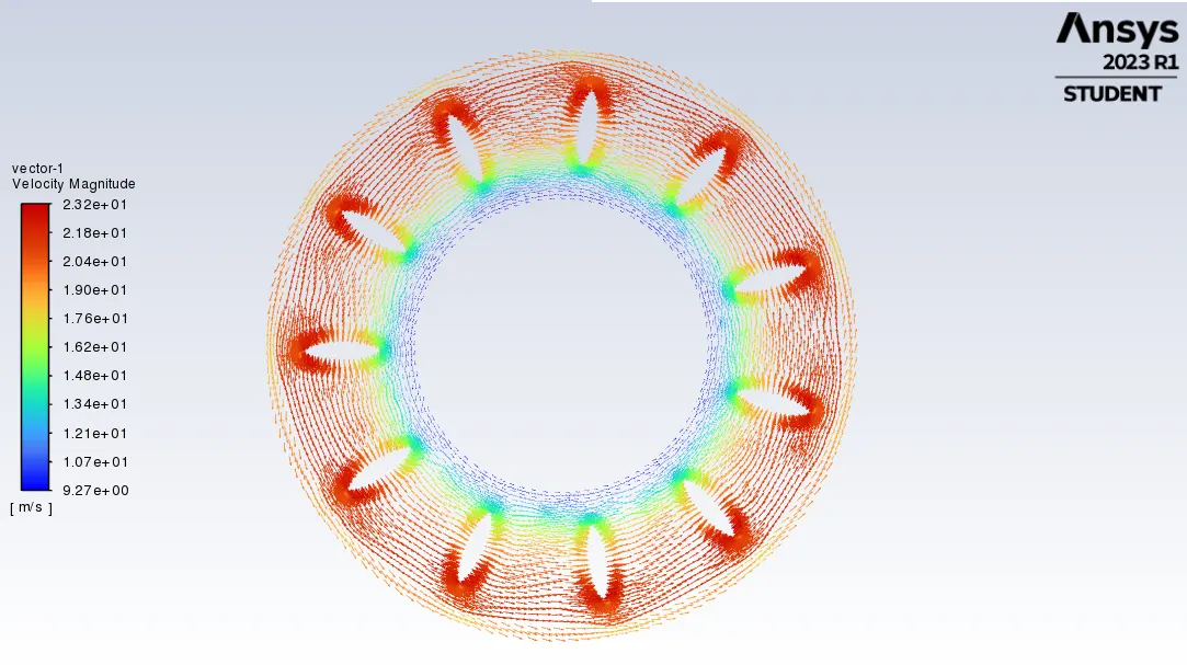
Plot the velocity profile and gradient, according to the results obtained from the simulation.

ENGINEERING DEVELOPMENT

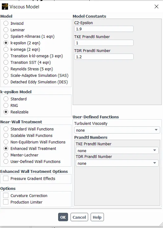
To start the simulation, the turbulence model is selected according to the statements of the challenge, being the `k-epsilon` Realizable model with enhanced wall treatment.

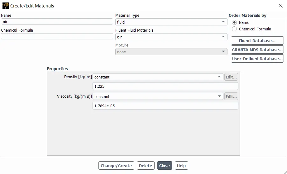
The fluid conditions are going to be air at standard conditions, these features are set by default.

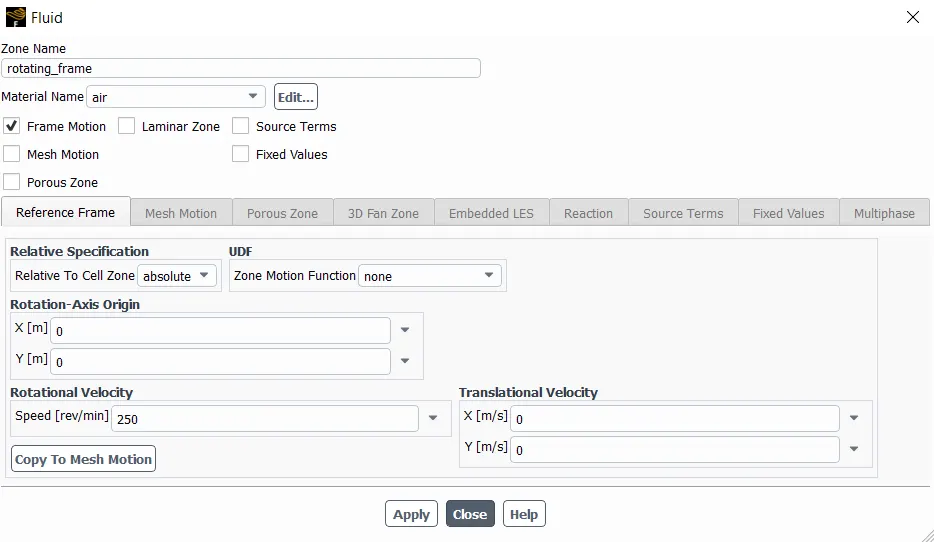
Now, to activate the frame motion, the fluid surface contains a function called "Frame motion", there, the rotational velocity appears, and the rotational velocity set for this simulation is equal to 250 rpm.

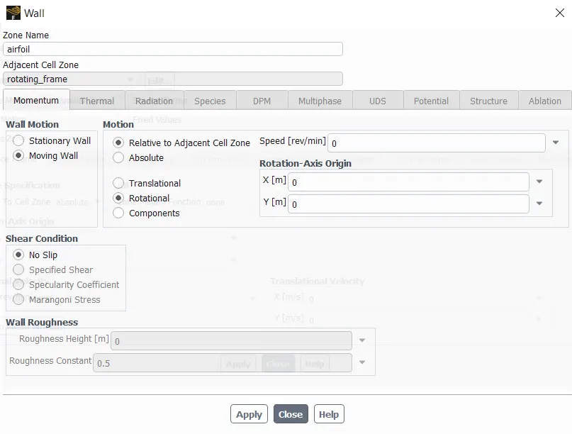
Likewise, the airfoil walls are also selected as moving walls, however, the motion of the airfoils is selected as rotational.

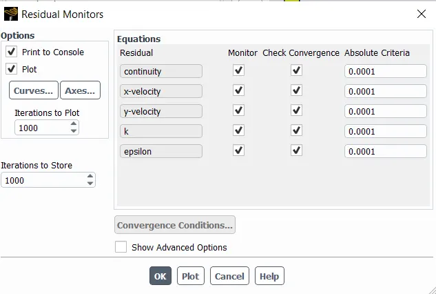
Once the physical parameters have been set, the next step is to settle the initialization parameters; the residuals are normally set by program default as 0.001, but in order to get more accurate results, the residuals are set as 0.0001.

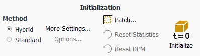
The initialization is performed by using a hybrid method to initialize the simulation.

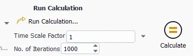
Finally, the simulation will be run with one thousand iterations.

RESULTS

The results obtained are:

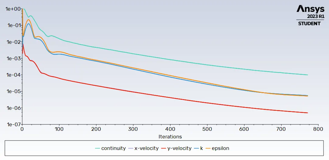
• Convergence

• Total pressure field

• Velocity profile

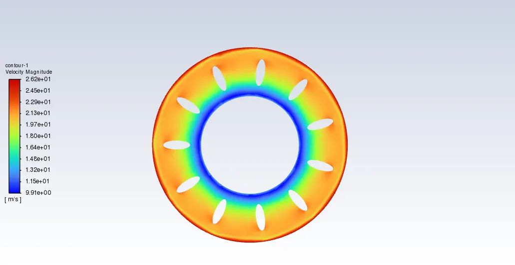
• Velocity gradient

CONCLUSIONS

The mixing plane model shows that the simulation reaches a good convergence and the profile plots are behaving accurately. However, in this case, convergence was obtained easily due to the domain does not have either an inlet or an outlet; then, to perform these types of simulations, the convergence of the simulation might take some iterations more.

The sliding mesh model was not required to get the simulation results, because of the rotating parts do not have a high interaction with the flow in this case.

REFERENCES

Chapter 9. Modeling Flows in Moving Zones, FLuent Inc. November 28, 2001.