Week 7 - Minor Project
NACA 0012 Airfoil Simulation
AIM
In the following project, the airfoil NACA 0012 will be simulated and analyzed by using ANSYS Fluent. NACA 0012 is considered in the industry as a thin airfoil that can be used to work from subsonic to supersonic flows because its shape is able to handle low-frequency shock waves. To perform each simulation, it will be used two meshes, previously created by using ICEM CFD (please review challenge 6 from this module for more information); then, the idea is to simulate the flow behavior around the airfoil by varying the angle of attack from this one, so that the velocity magnitude at each axis must be calculated.
Furthermore, the turbulence model has to get accurate results, to achieve that, it must be carried out literature research about the turbulence model normally used for simulating airfoils; all these documents will be referenced below. Finally, the lift and drag coefficients obtained from incompressible flow simulations are going to be compared with the values obtained from the compressible flow simulations.
EQUATIONS
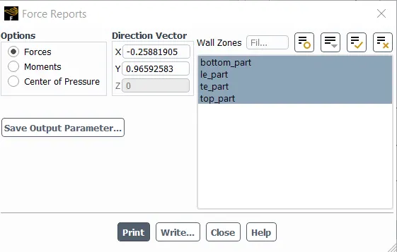
Lift vector
`X=-sin(alpha)`
`Y=cos(alpha)`
Drag vector
`X=cos(alpha)`
`Y=sin(alpha)`
Where `alpha` is equal to the angle of attack of the airfoil.
OBJECTIVES
Determine the velocity magnitude in each axis, according to the statements imposed by the project as incompressible as compressible flow.
Research for the best solver type and fluid conditions to get more accurate results once the simulation has been performed.
Analyze the drag and coefficients obtained from each analysis, in order to determine whether these aerodynamic coefficients remain constant with the speed increasing and just change once the angle of attack is varied.
ENGINEERING DEVELOPMENT
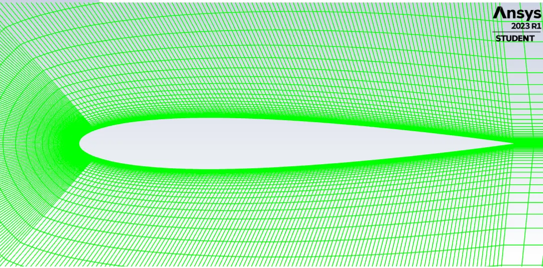
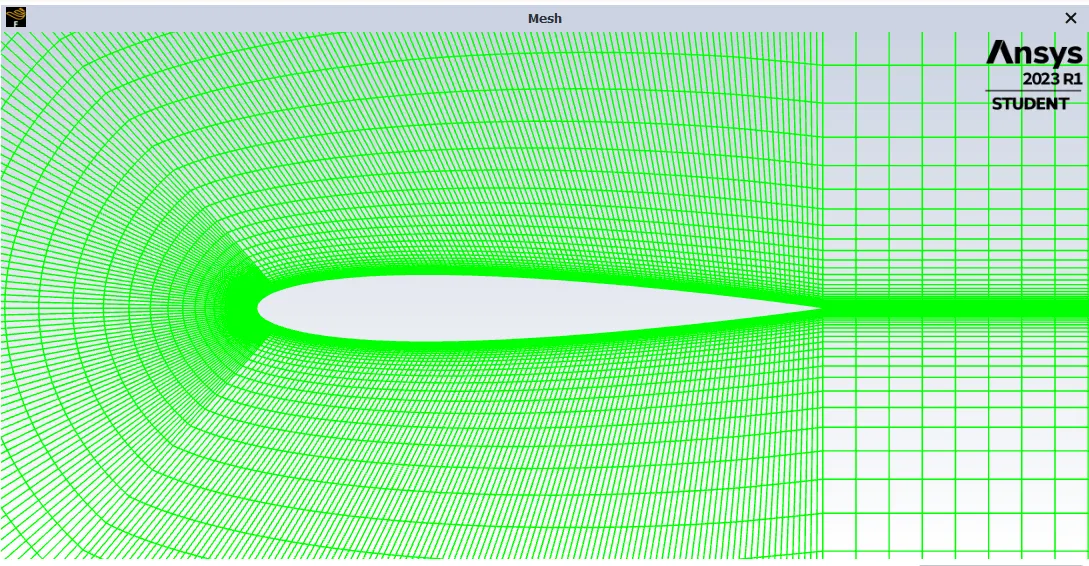
Initially, two meshes are created by using ICEM CFD, because the mesh in compressible flows must have a lower aspect ratio in each cell, to get more accurate results in the sections where shock waves are generated; in the following two pictures, the difference of the mesh at the rear section of the airfoil can be noticed. The mesh files are also attached at the end of this project.
Incompressible flow
Compressible flow
Then, the airfoil will be simulated with 5, 10, and 15 degrees of angle of attack; so that the velocity magnitude at each axis will have the values shown on the table below.
| Incompressible | Compressible | |||
| Angle of attack | X Velocity (m/s) | Y Velocity (m/s) | X Velocity (m/s) | Y Velocity (m/s) |
| 5 | 51.9516 | 4.5452 | 270.965 | 23.706 |
| 10 | 51.3571 | 9.0558 | 267.868 | 47.232 |
| 15 | 50.3730 | 13.4974 | 262.732 | 70.399 |
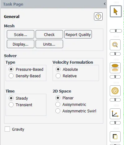
The solver selected to perform all the simulations is about Pressured-based, even for compressible flow. This one is selected due to the Density-based solver is commonly used for compressible flows, however, Density-based solver mainly works for fluids where the shock wave is remarkable, being at Mach 2.5 or greater.
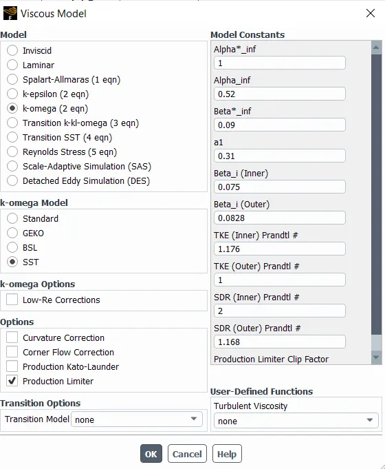
Likewise, the turbulence model will always be `k-omega` SST model, because this model can get the flow behavior over the near-wall more accurately than the other models. It has to be considered that the energy equation must be activated at the moment when the compressible flow analyses are going to be carried out.
The first wall cell-height is `1.6*e^-6`for the incompressible flow mesh, and `7.4*e^-6`for incompressible flow.
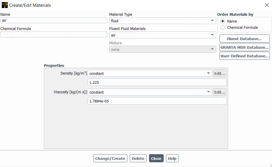
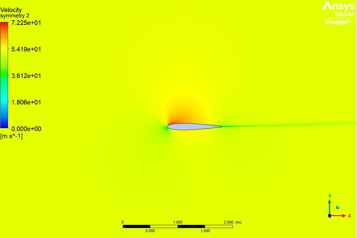
Now, the flow features for the two cases are shown below. This won't be changed in any of the cases.
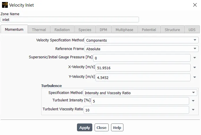
The next step is to put the velocity magnitude at each axis, according to the table attached above; in ANSYS Fluent the velocity method must be changed to "Components" and the tool box will show the velocity inputs as is shown in the following picture.
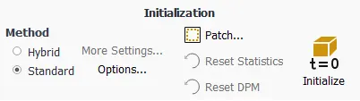
Furthermore, the solver method will be Standard and the field features will be calculated from the inlet section.
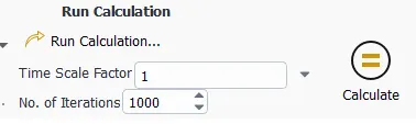
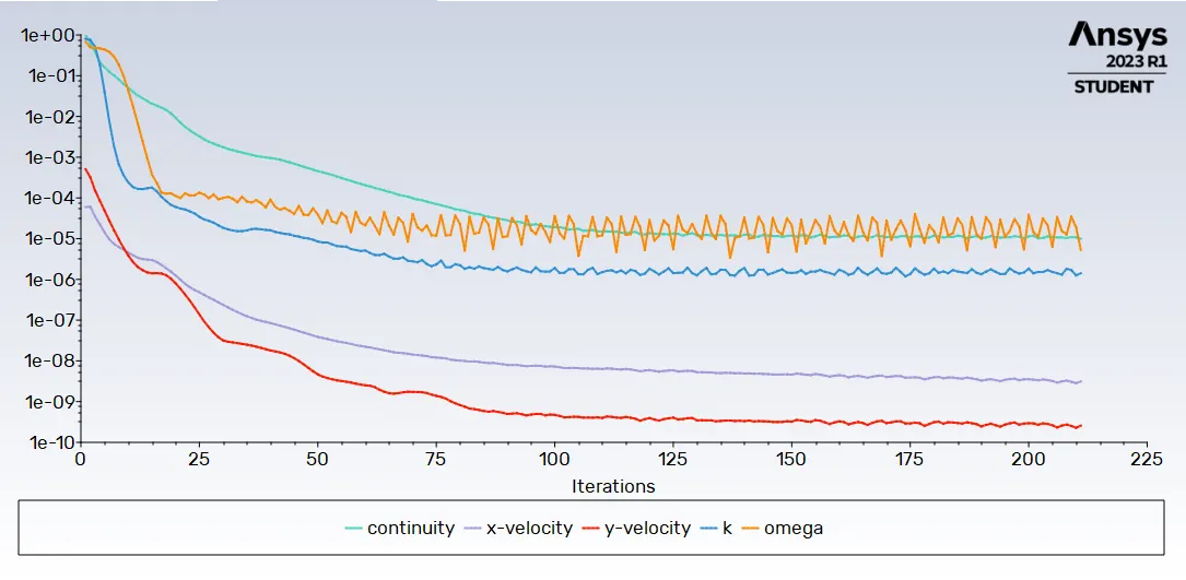
Finally, to get the convergence of the model parameters, the number of iterations is taken until one thousand iterations. any other simulation parameter must not be changed.
To obtain the lift and drag coefficients, the equations described above must be used, due to the program throws the values aligned to each axis, which are not the accurate values.
RESULTS
The results obtained from each simulation have been classified in order to show:
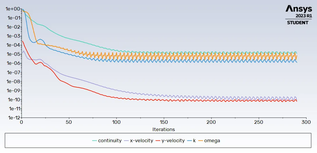
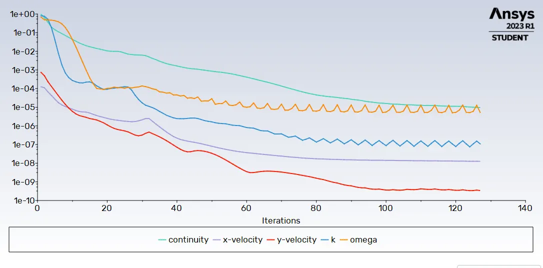
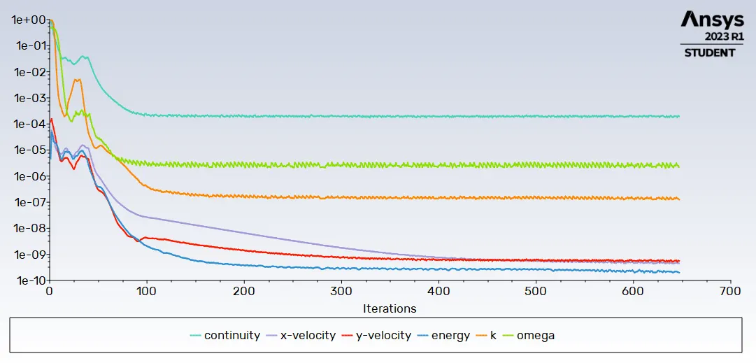
a) The convergency of the simulation;
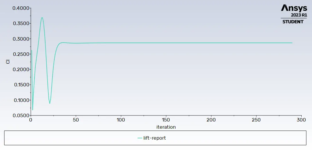
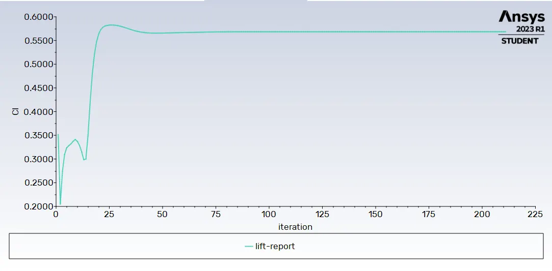
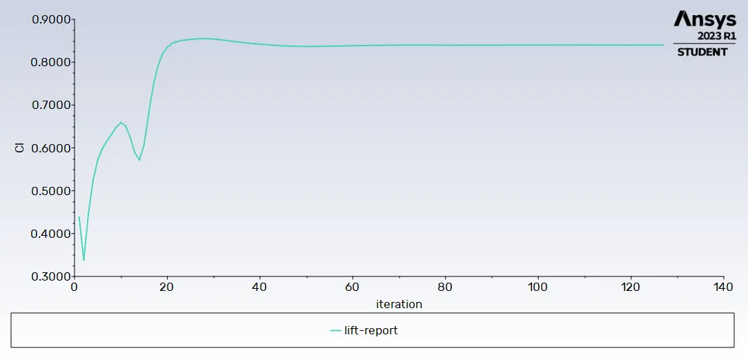
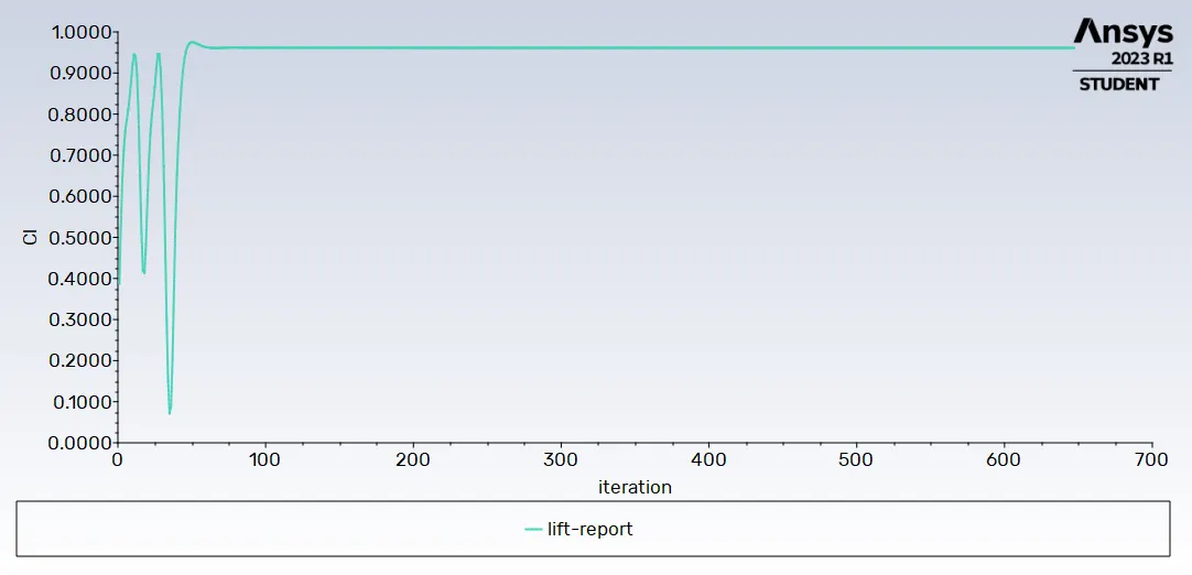
b) The lift coefficient behavior in each iteration;
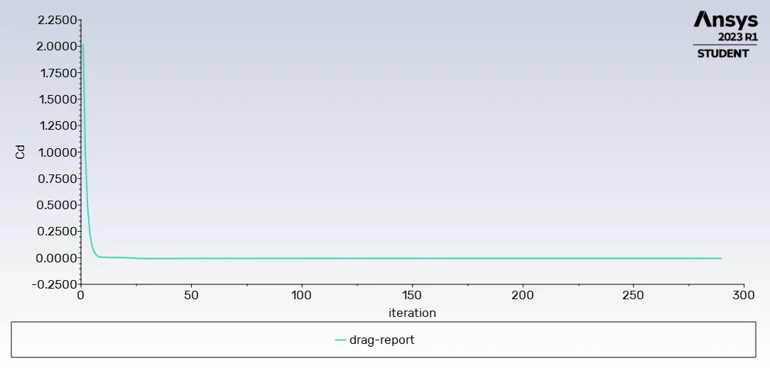
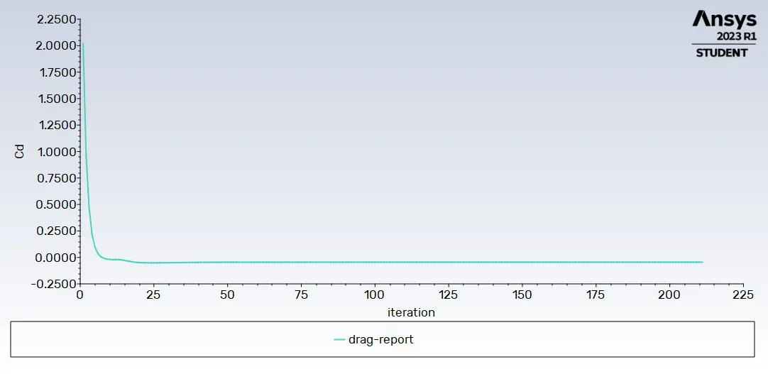
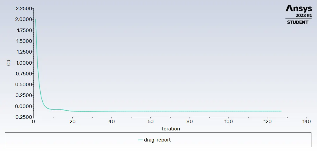
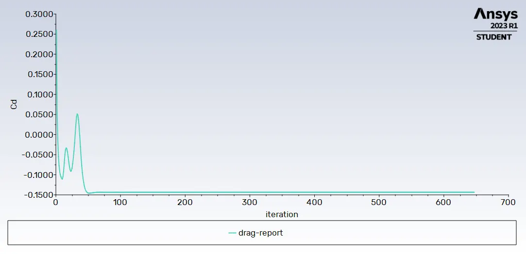
c) The drag coefficient behavior in each iteration;
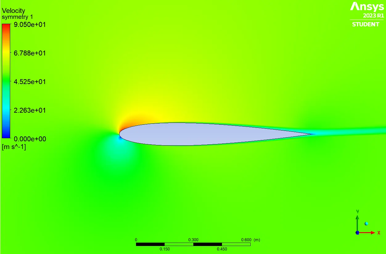
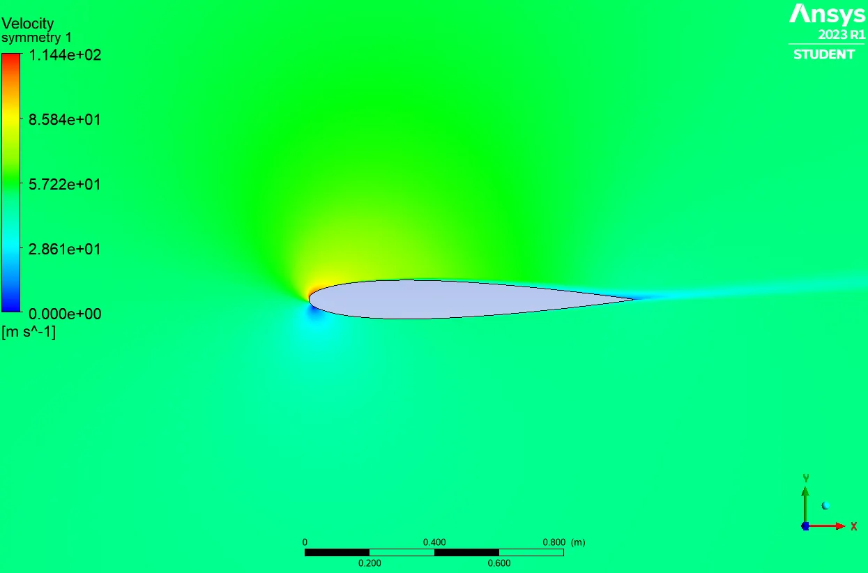
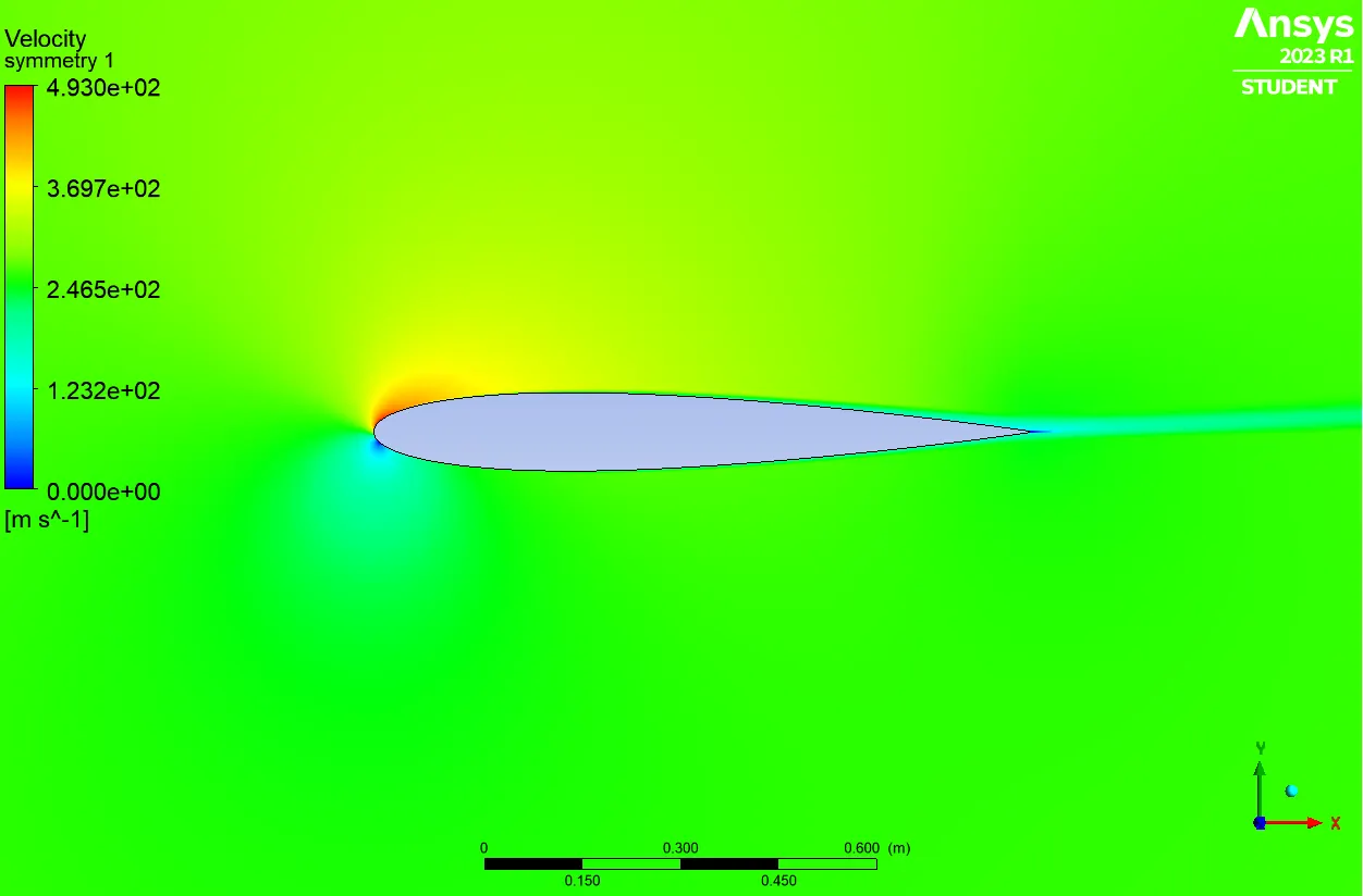
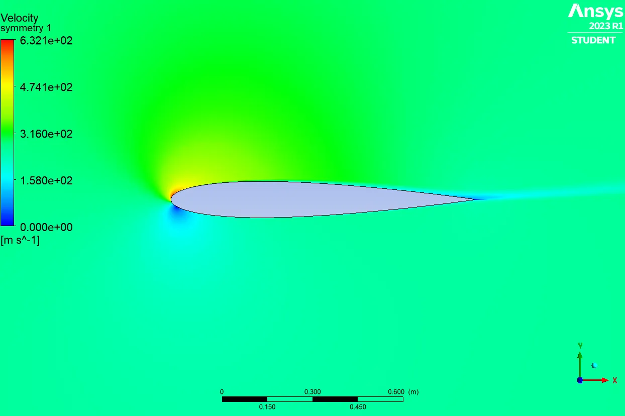
d) The velocity field around the airfoil, and;
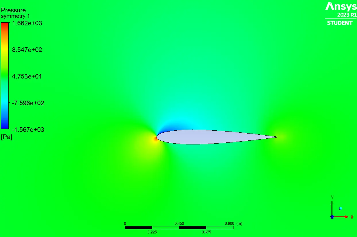
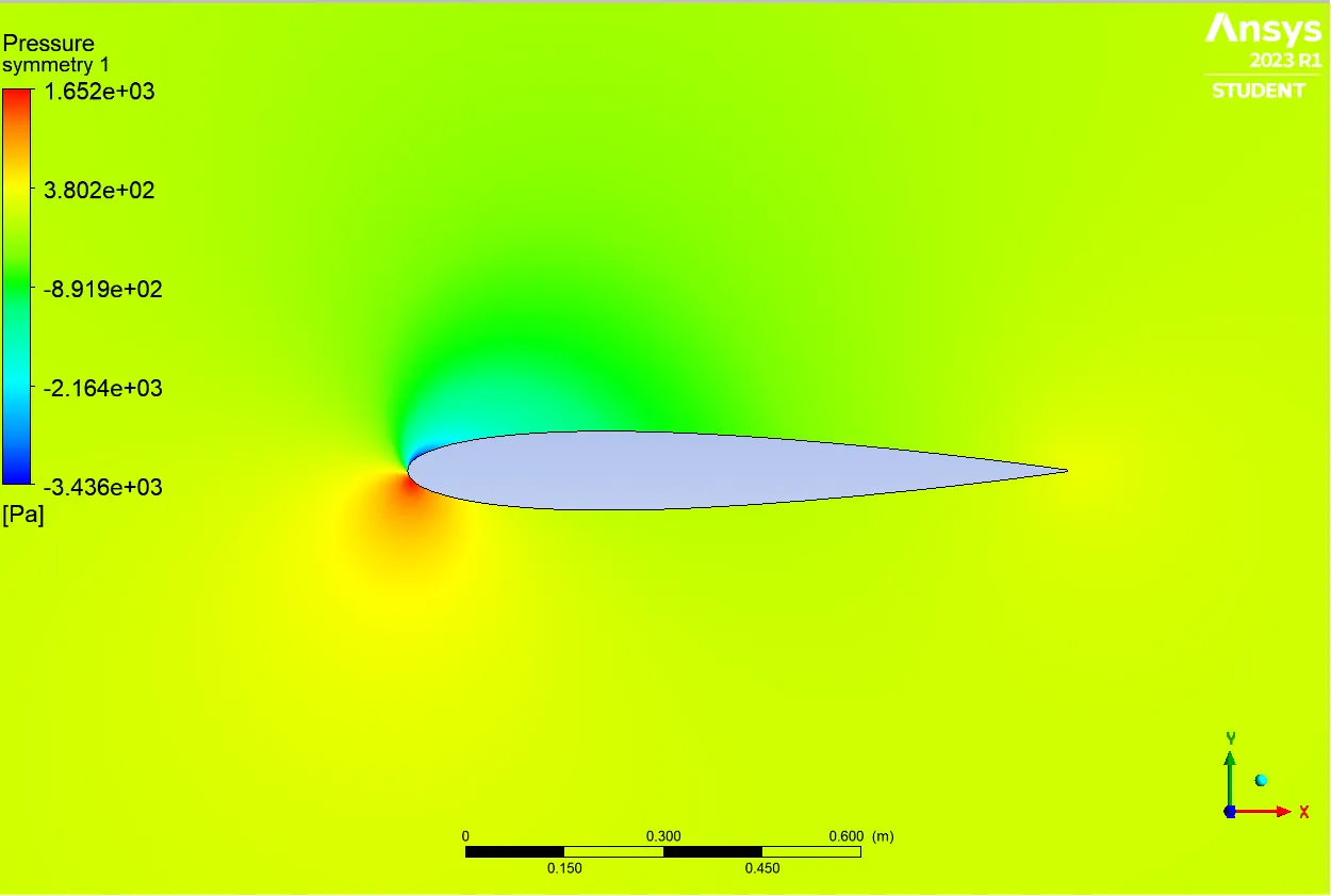
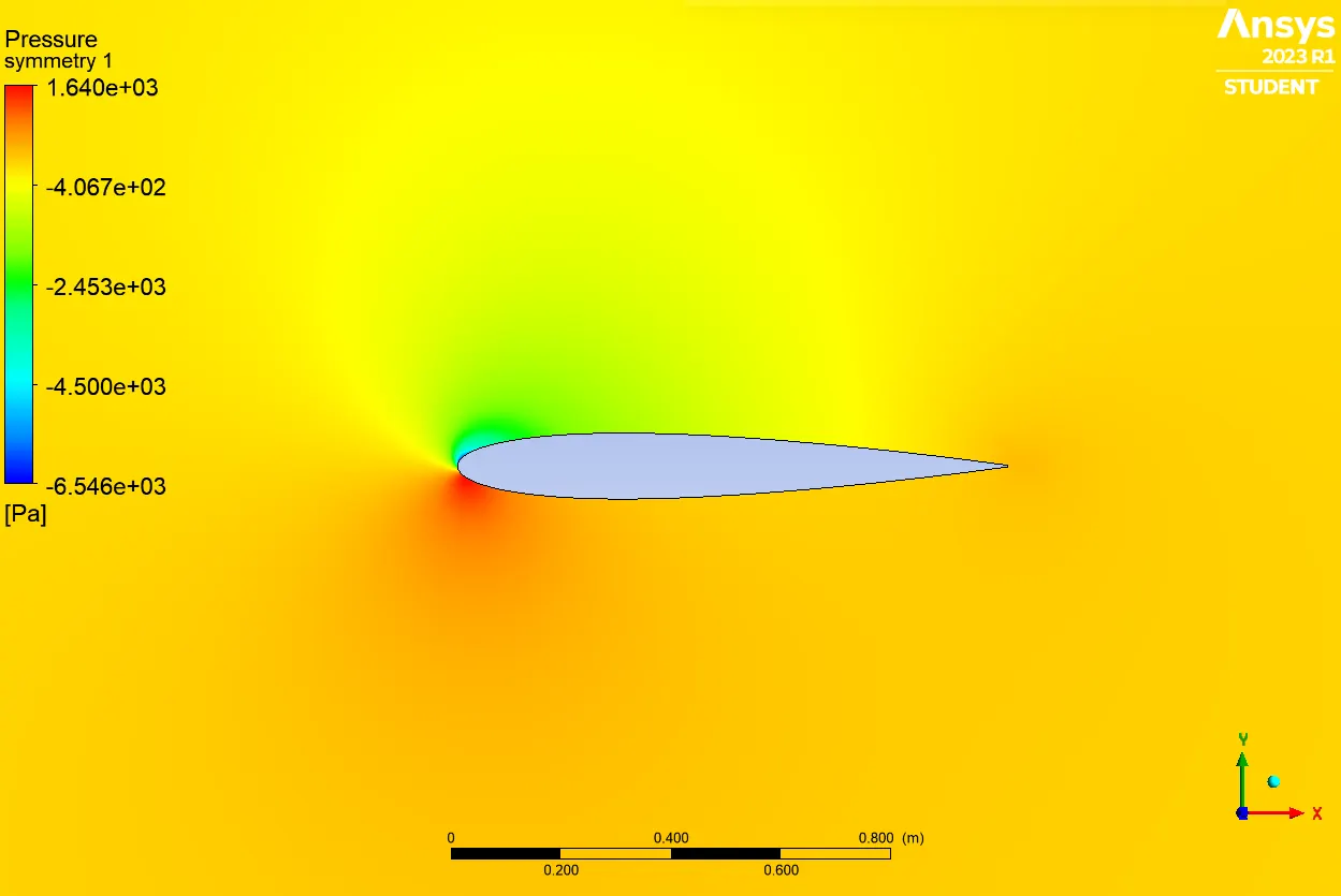
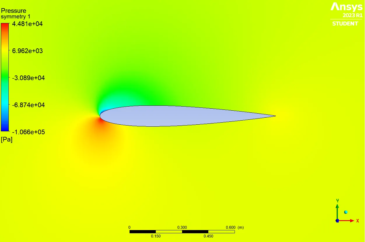
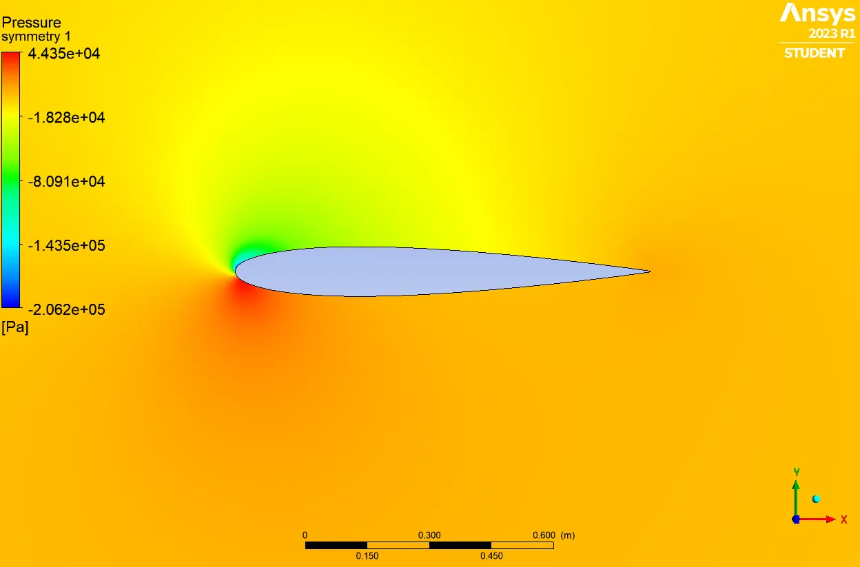
e) The pressure field around the airfoil.
- Subsonic regime
1. Angle of attack: 5°
- Convergency
- Lift coefficient
- Drag coefficient
- Velocity field
- Pressure field
2. Angle of attack: 10°
- Convergency
- Lift coefficient
- Drag coefficient
- Velocity field
- Pressure field
3. Angle of attack: 15°
- Convergency
- Lift coefficient
- Drag coefficient
- Velocity field
- Pressure field
The average coefficient values obtained for each simulation are:
| Angle of attack | Lift coefficient | Drag coefficient |
| 5 | 0.286 | 0.0204 |
| 10 | 0.568 | 0.054 |
| 15 | 0.8406 | 0.1076 |
- Supersonic regime
1. Angle of attack: 5°
- Convergency
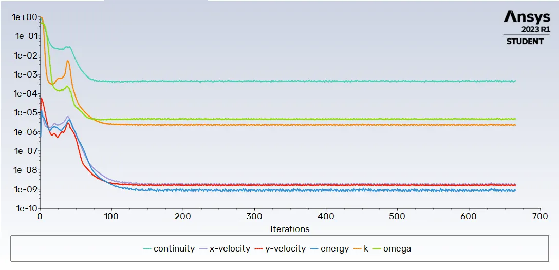
- Lift coefficient
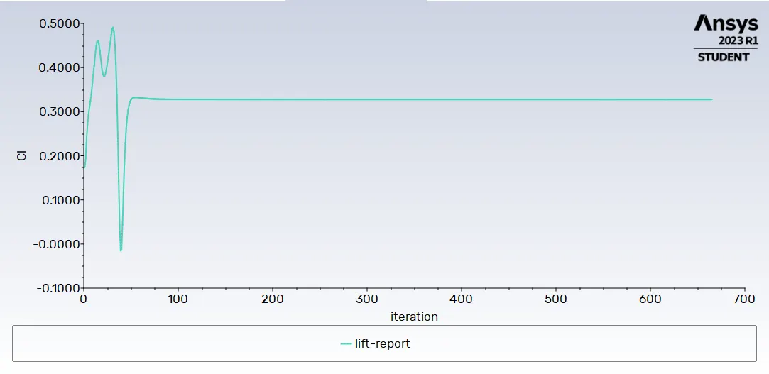
- Drag coefficient
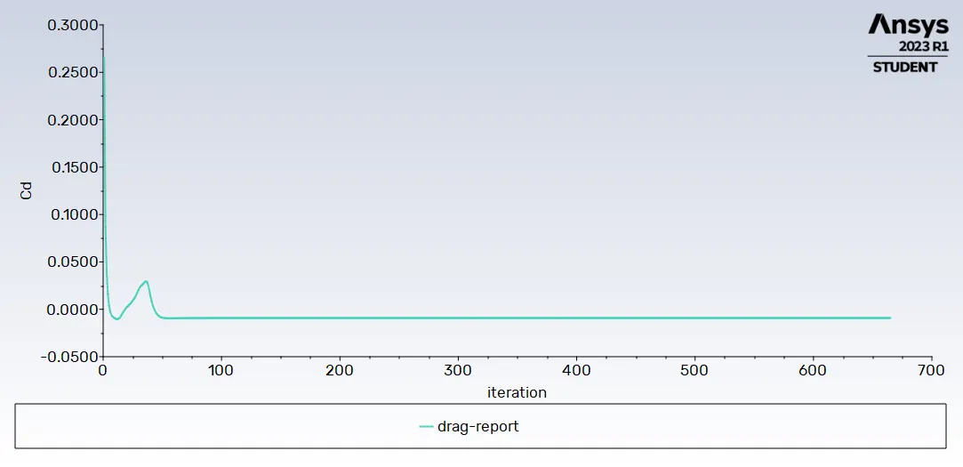
- Velocity field
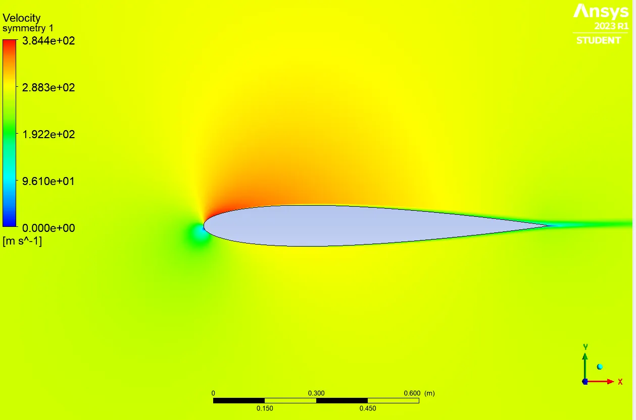
- Pressure field
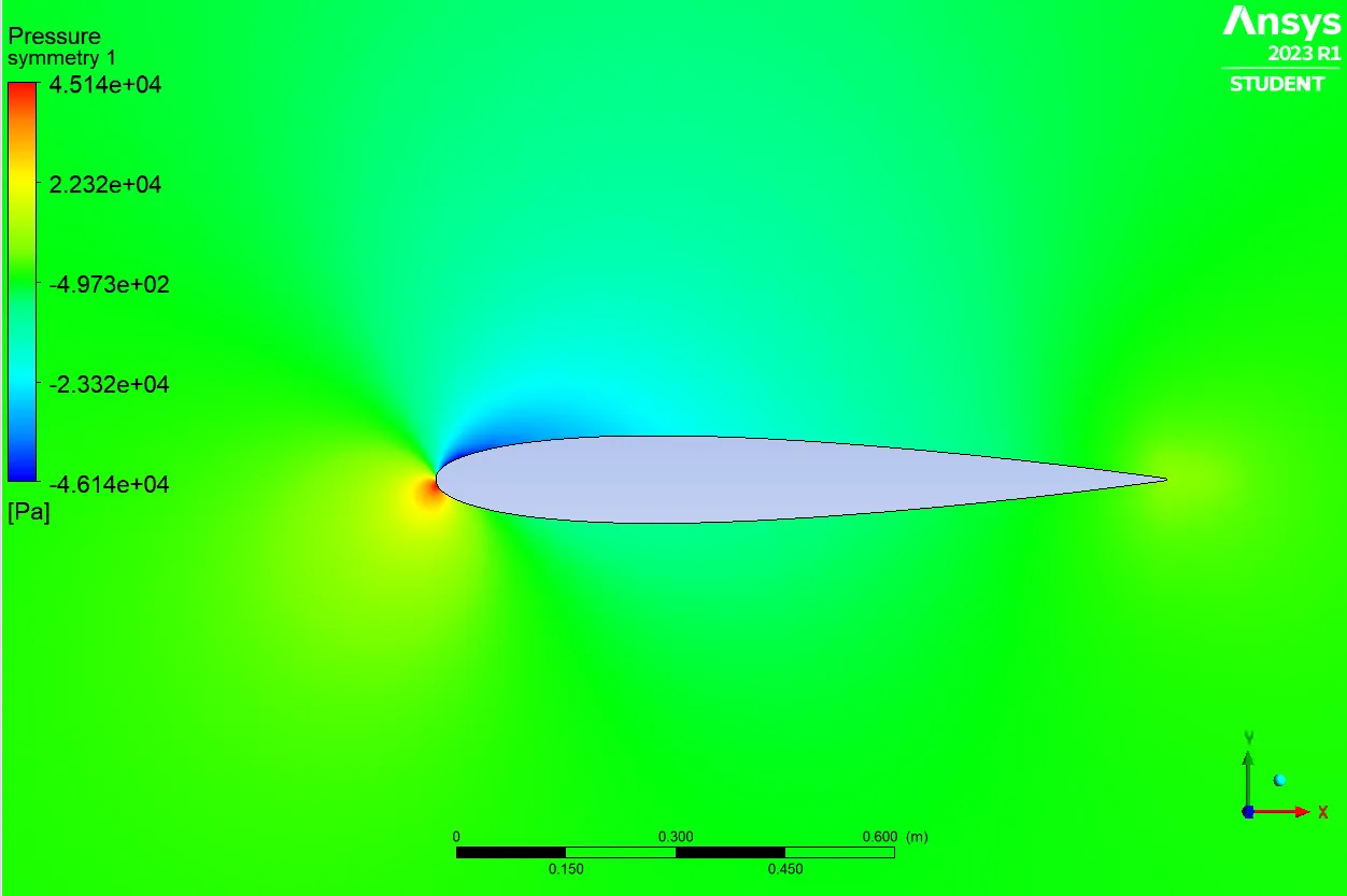
2. Angle of attack: 10°
- Convergency
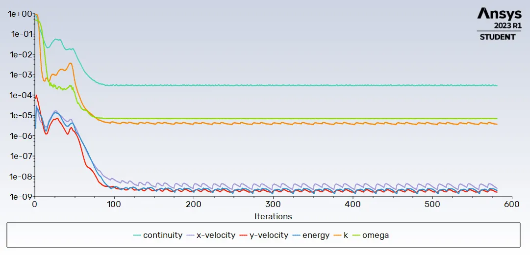
- Lift coefficient
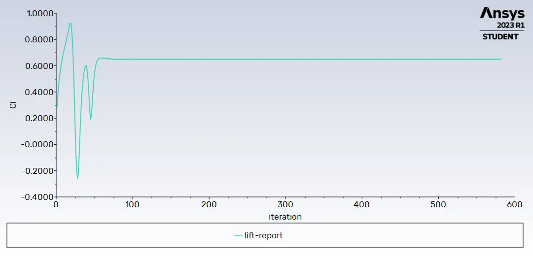
- Drag coefficient
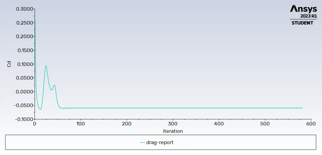
- Velocity field
- Pressure field
3. Angle of attack: 15°
- Convergency
- Lift coefficient
- Drag coefficient
- Velocity field
- Pressure field
Similar to the incompressible flow simulations, the coefficient values thrown by the program are:
| Angle of attack | Lift coefficient | Drag coefficient |
| 5 | 0.3272 | 0.0194 |
| 10 | 0.6503 | 0.0544 |
| 15 | 0.9655 | 0.11 |
Thus, it can be determined that the lift and drag coefficient on airfoils just significantly change if the angle of attack at which the airfoil is facing the flow is varied; the lift and drag coefficient at five degrees of angle of attack are very close to each other in an incompressible and compressible flow, nevertheless, the coefficient values obtained between five and ten of the angle of attack differ too much.
CONCLUSIONS
The drag and lift coefficients in airfoils will only depend on the angle of attack at which the airfoil is being dived into the flow, rather than another primitive parameter. However, the flow speed and other features will make the coefficients obtained differ a little because the flow will behave differently as the top as the bottom airfoil surface, due to the differential pressure and the change of the density becomes an important feature that affects the flow behavior.
It can be seen that the lift coefficient tends to increase once the angle of attack is increased too; however, it cannot be assumed that the lift will continue increasing more and more, because of the increase is achieved according to the Coanda effect and the differential pressure below the airfoil. It must also be taken into account that the drag coefficient is increasing in a parabolic way; so that the airfoil will enter into the stall performance if the drag coefficient increases more than the lift coefficient.
The drag coefficient increases considerably once the angle of attack increases, due to the flow is separated faster than in low angles of attack; therefore, the flow separation might occur easier in greater angles of attack and the airfoil could get the stall performance in a determined angle of attack. For this airfoil, the stall angle of attack is greater than approximately 19 degrees.
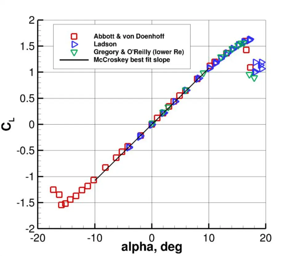
Image taken from:https://turbmodels.larc.nasa.gov/naca0012_val.html
REFERENCES
https://www.hindawi.com/journals/mse/2011/714146/
https://me.buet.ac.bd/icme/icme2001/cdfiles/Papers/Keynote/18_Shirani_final.pdf