Week 4 - CHT Analysis on Exhaust port

CHT Analysis on Exhaust port report

AIM

The following project will be developed in order to determine thermal characteristics on an exhaust port which is taking hot flow out. it will be firstly calculated the wall distance heigth that the neghbor mesh cells should have to simulate the turbulence over the inner exhaust walls. Then, it will be prepared and refined as the exhaust geometry as the body meshing; once these two steps have been concluded, it will be entered the physical features that the fluid and solid will have and it will be finally simulated and analyzed the flow and body behavior at this kind of physical exposure.

This project will have a particular analysis known as CHT analysis (Conjugate Heat Transfer), where the CHT is calculated over the whole body, using ANSYS Fluent to get easily these values. CHT analysis is commonly used to determine issues as hottest points in thermal reactors, jet engines, electronic devices, nuclear power reactors, etc. Besides analyze those issues, CHT is also used to predict the material resistances exposed under abrupt temperature changes, where some material regions suffer even more than others and due to that, the material could change its mechanic properties. Thus, it is clear the HTC analysis is used in almost all engineering fields where the temperature might be a concern.

In this project the CHT analysis will be shown by using hot flow passing though a exhaust port with a determined material, such that the fluid will deliver thermal energy to the exhaust body, but this energy values will differ regarding the flow keeps going moving along the inner exhaust.

EQUATIONS

• Reynolds number:

`Re=(rhoVl_h)/mu=(rhoVD)/mu`

where:

`mu=`fluid dynamic viscosity

`rho=`fluid density

`D=`mean pipe diameter

`V=`flow velocity

• Friction coefficient - Internal flow:

`c_f=0.079*Re^(-0.25)`

• Wall shear stress:

`tau_w=1/2V^2rhoc_f`

• Frictional velocity:

`u_t=sqrt((tau_w)/rho)`

• Wall heigth distance:

`Deltay= (vartheta*y^+)/u_t`

where:

`y^+=`dimensionless cell heigth (less than 5 on the viscous layer)

• Heat transfer coefficient:

`h=q/(T_(wall)-T_(ref))`

where:

`q=`transfer heat

`T_(wall)=`Wall temperature

`T_(ref)=`Reference temperature - fluid temperature

OBJECTIVES

• Prepare the geometry and refine the mesh around and inside the geometry.
• Simulate the flow behavior into the exhaust port, taking into account the wall heigth distance in order to get an accurate solution.
• Determine the highest heat transfer coefficient along the exhaust walls and the accuracy of the results obtained.

ENGINEERING DEVELOPMENT

To start the simulation which will be carried out on the exhaust port provided by the challenge statements, it is necessary to get the main conditions that they are going to get certaincy the simulation will get the most accurate results. In order to reach such accurancy, it is required to determine the wall distance heigth and take into account the best turbulence model according to the researches theory.

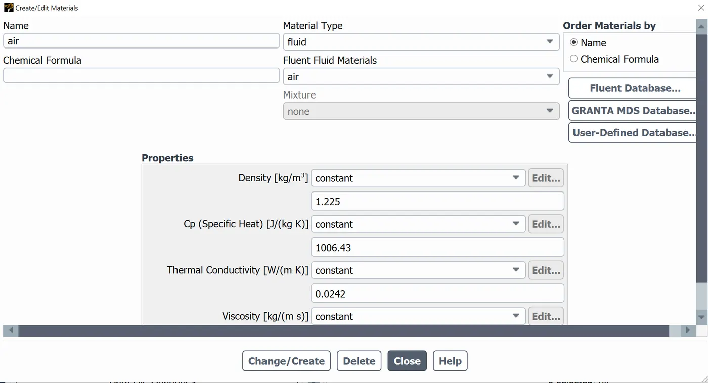
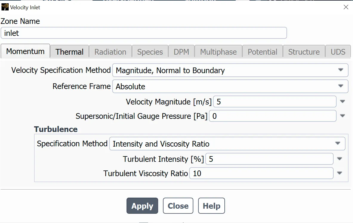
So, the equations set above will serve for determine the wall distance heigth; Firstly, it is known the fluid and the flow speed, being air at 5 `m/s`. Air properties are exposed below on the "Fluid features" picture and, the mean characteristic length between the inlet and the outlet diameters would be `D= 0.15805 m`. Thus, the reynolds number will be equal to:

`Re= 54111.6`

Then, the friction coefficient, wall shear stress and frictional velocity can be also calculated, using the reynolds number obtained; It must be noticed the friction coefficient equation have to be the equation for internal flows. The results obtained are:

`c_f=0.00518`

`tau_w=0.07932 Pa`

`u_t=0.2545 m/s`

Finally, assuming the `y^+` value is equal to 1 on the viscous layer, the wall distance heigth will be then equal to:

`Deltay=0.0581532 mm`

Once the wall distance heigth at the first mesh grid over the inner wall is calculated, the geometry preparation is carried out on ANSYS Spaceclaim. It has to be used "Volume extract" to get the internal geometry which will be taken by ANSYS as the fluid portion into the goemetry.

It is then joint the to geometries obtained in a one component, in order to use a practical tool provided by ANSYS, known as "Share". The icon "share" serves for rearranging the mesh cells between internal surfaces of the exhaust and the external surfaces of the fluid body; using this tool, the mesh cells on these two boundaries will aligne their nodes with each other and the final mesh at the cross-section will look like the mesh shwon in the third picture below. To be sure the share arrangement was applied on the geometry, the purple circles shown on the two pictures below must be plotted by the program.

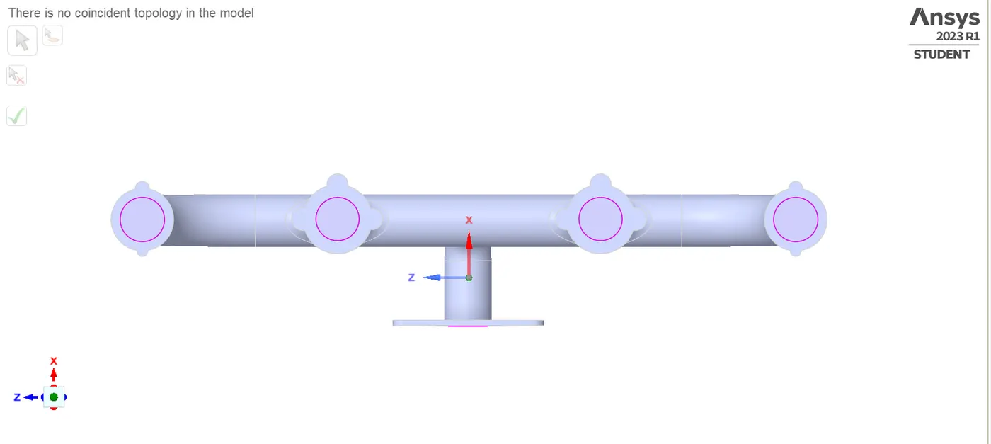
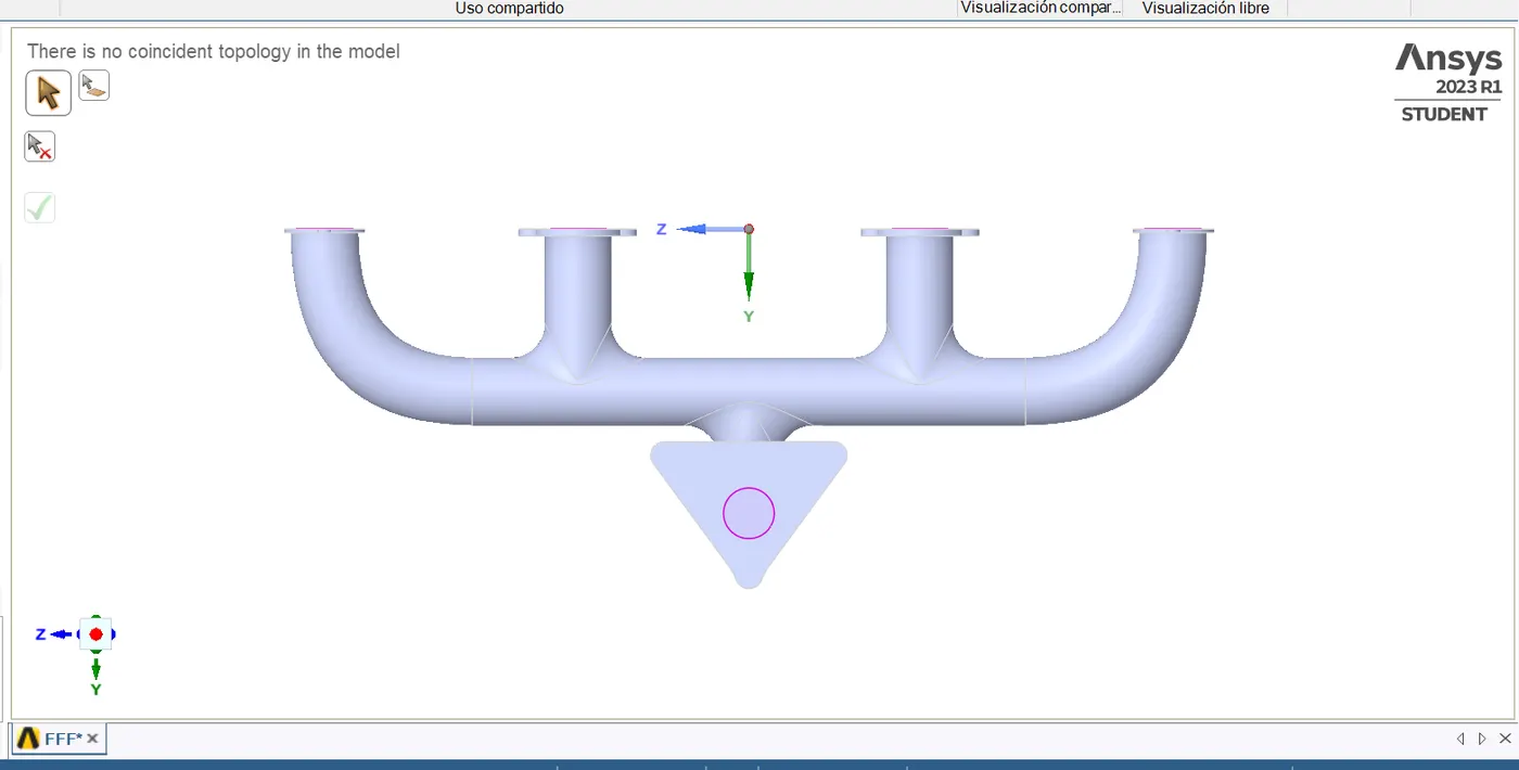
Now, if the share icon was used succesfully, the mesh cell around the cylinder geometry should look like as it was described above. All the mesh cells around the outer body and fluid body have their nodes joint, making sure the values into these cells will not trigger innacurate results due to the lack of the mesh alignment. Take into account that if the mesh are not aligned, the result on the fluid body region boundary and on the body wall boundary might not share the same information.

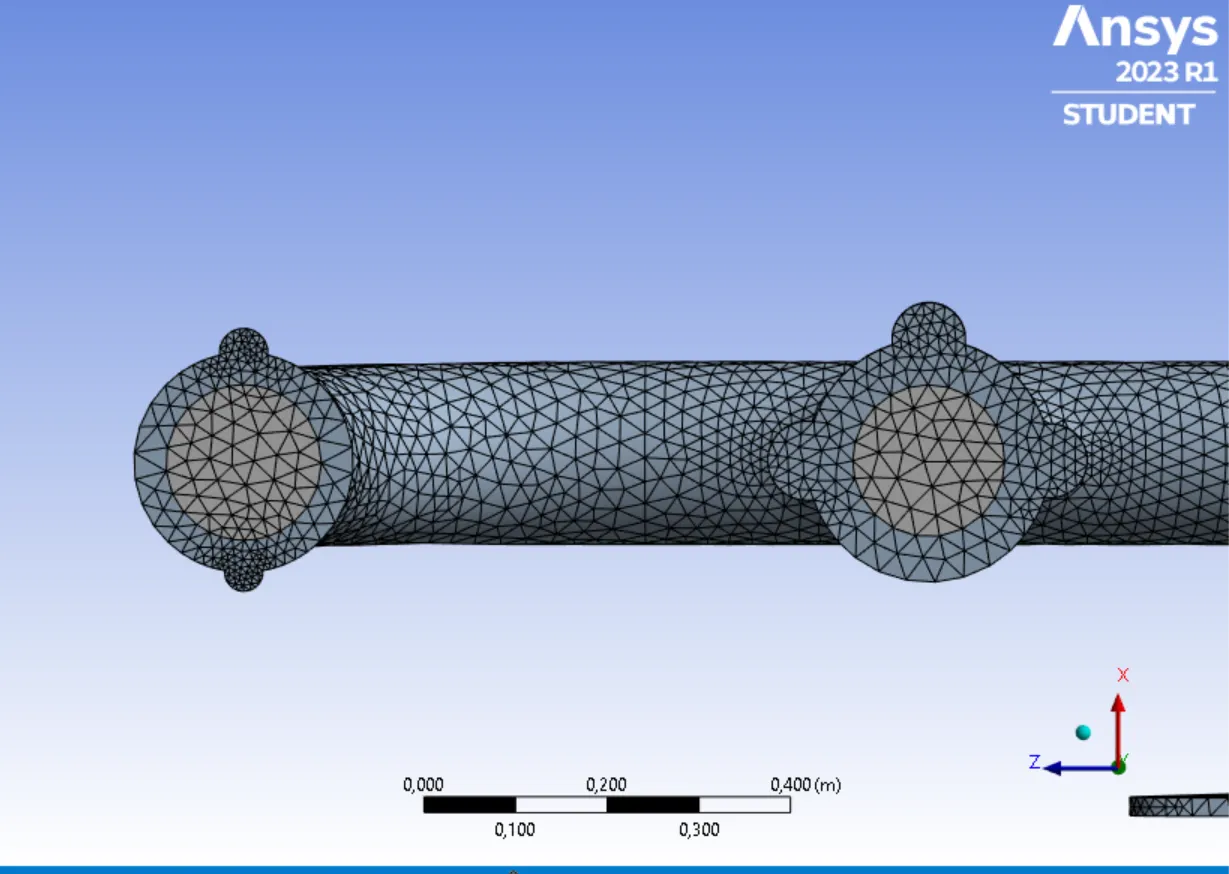
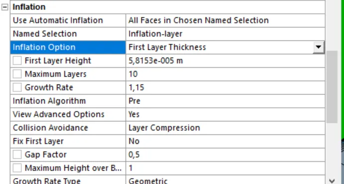
Besides generate the mesh on the exhaust and fluid bodies, it is also named the external fluid layer, to refine the mesh around these surfaces, so that the wall distance heigth can already be set over the inner exhaust walls.

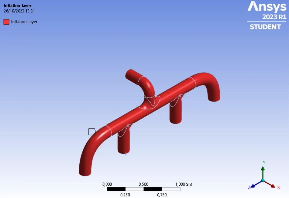
In the picture below, it is shown the first mesh over the inner walls will have the heigth calculated. Furthermore, the growth hiegth of the next 10 mesh cells near the wall, will have an increasing of 15% from the wall distanceheigth value.

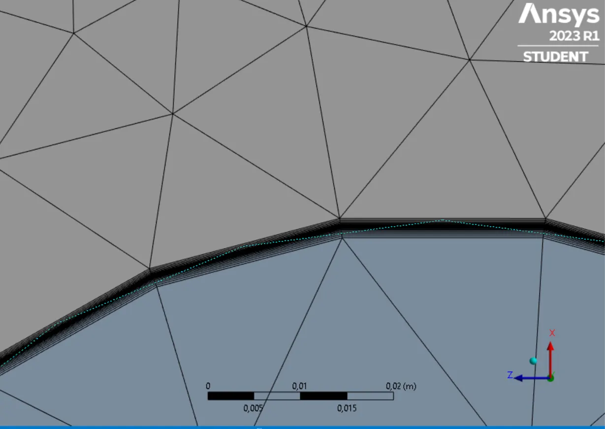
The mesh refinement result will look like it is shown in the following picture.

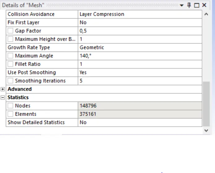
Two more refinements steps are carried out over the main component and the whole body, using a mesh size of `30mm`on the exhaust body and a mesh size of `60 mm`on the entire body. It is obtained the following mesh statistics:

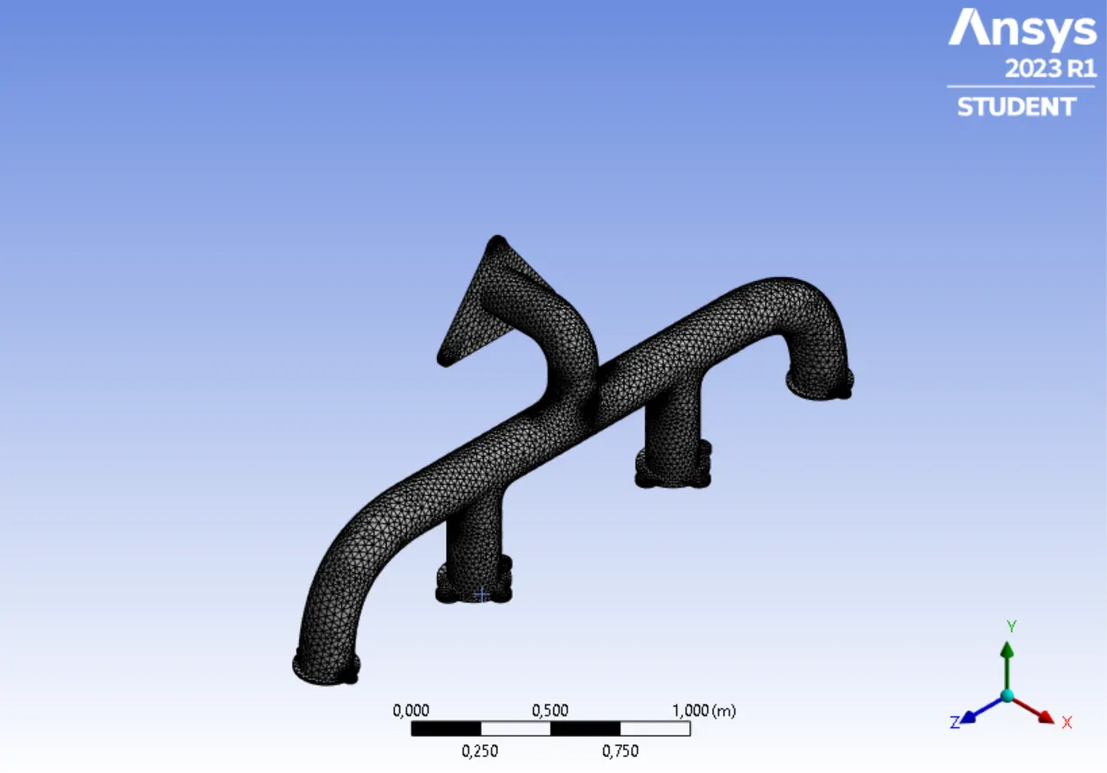
The final mesh is plotted as the image below.

The next step is to define the physic parameters and the appropiate model which will make sure the simulation will obtain an accurate results. To make this, it was required to get a turbulence model according to the research theory, where it is clear that there are two possible models which achieve to get the most accurate results for internal flows. The first one and most common is `k-epsilon` model , using scalable wall functions , because of the mesh refinement is carried out , assuming the `y^+`value is less than 11.25. (Information taken from: https://lms.skill-lync.com/programs/94933/23/choosing-a-right-turbulence-model/knowledgebase)

Then, `k-omega`SST model could be used too, using curve correction (tool provided by ANSYS Fluent), due to this model is good solving internal flows, separated flows and jets models, obtaining an accurate results for high pressure gradients. (Information taken from: https://forum.ansys.com/forums/topic/difference-between-k-epsilon-and-k-omega-turbulence-model/)

In this case will only be used `k-epsilon`model for scalable wall functions.

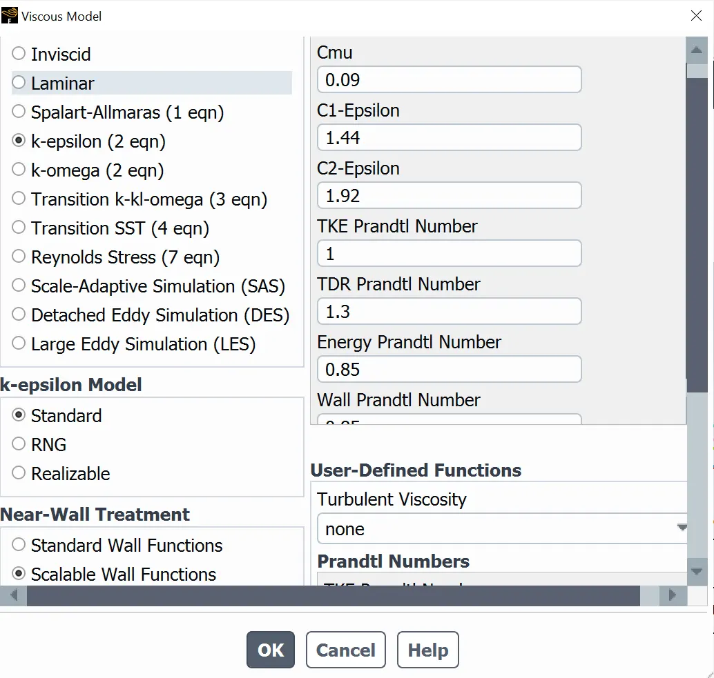
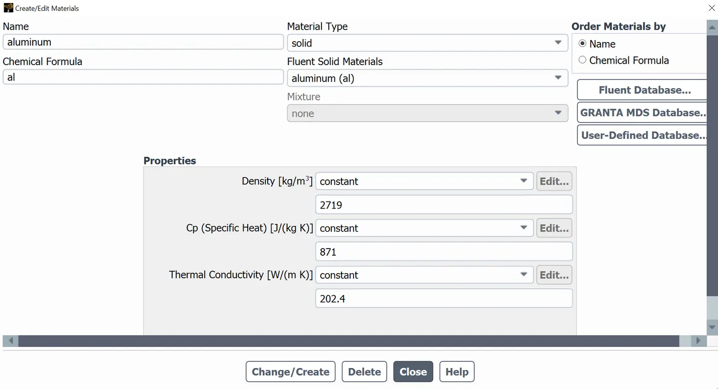
Likewise, the components will have different material features, taking the fluid as air and solid exhaust as aluminum.

• Fluid features:

• Solid features:

Inlet section are the four holes distribution that it can be seen on the exhaust geometry, the speed which the flow gets into the exhaust was defined above and the flow temperature will be equal to 700K.

The wall features except the external handles that are attached out of the inlets and outlet sections will be:

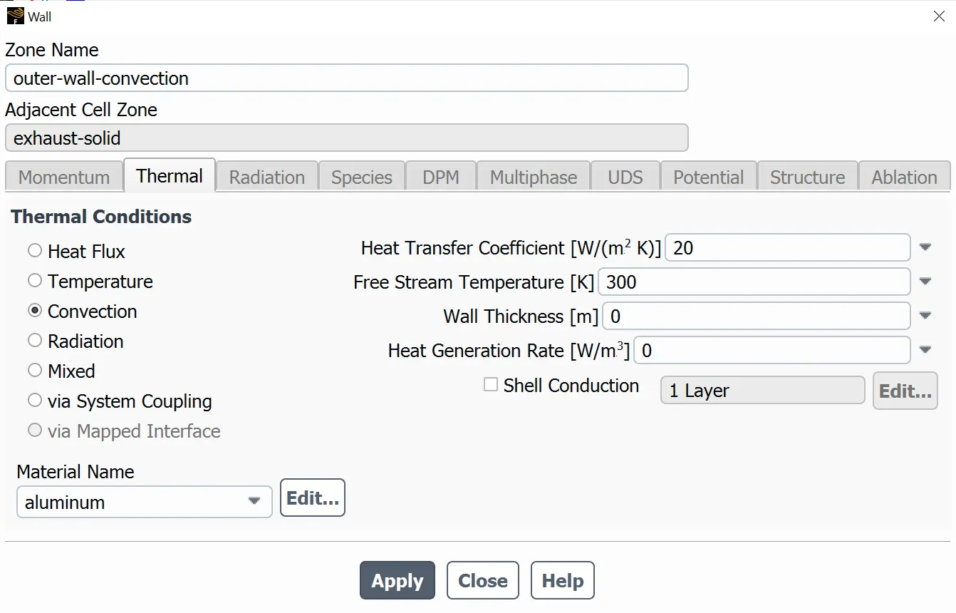
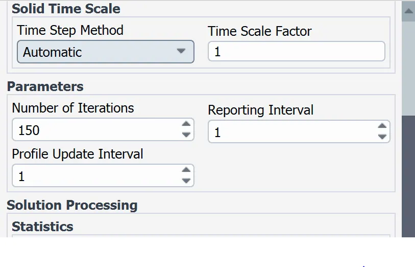
Finally, the number of iterations to obtain an a good accurate approximation will be 150. It is set on the calculate section and the simulation is ran.

RESULTS

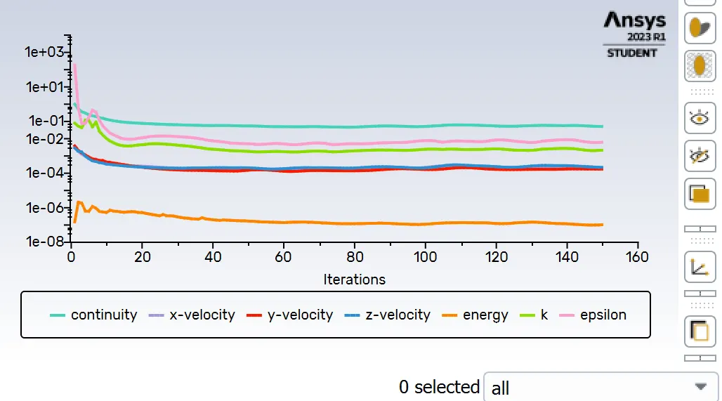
The convergency obtained is shown in the following picture. It can be seen the values achieve to keep an alike result, where the presicion of the values does not differ.

• Convergency plot:

However, it is now necessary to review the results obtained in the simulation, where the values should be approximated to a real value. To do that, it is necessary to compare the results with expermient cases where the flow would accomplish the same features which have been used in this simulation. This kind of simulation is only obtained by the students that have performed the same project on Skill-lync, due to that, the results comparison will be performed according the results obtained by two different student projects. (Student project is referred at the end of this project)

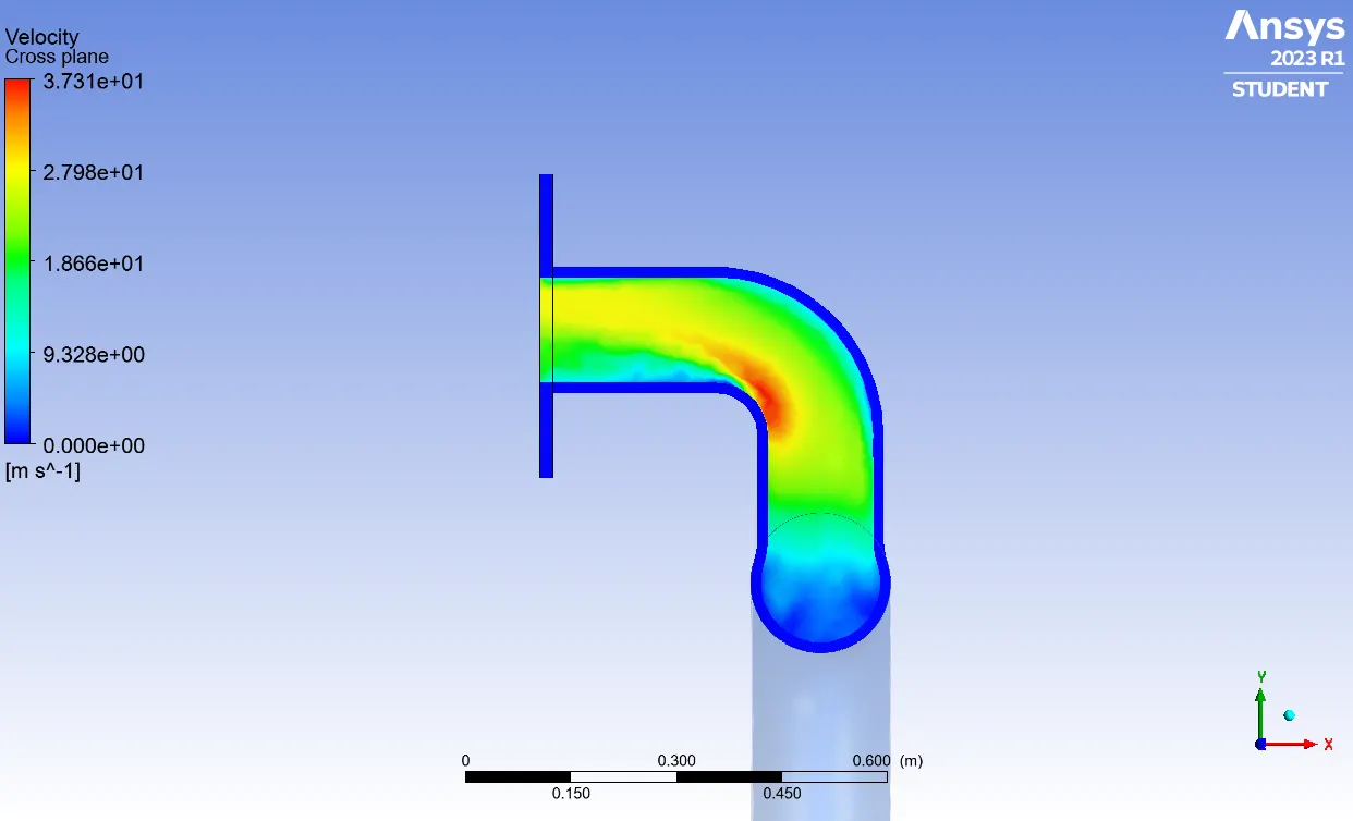
Velocity and heat transfer coefficient are correlated because of the convective transfer heat and conductive transfer heat are both related with the Nusselt number, which is also related with the Reynolds number and Prandlt number. So, if the flow speed is great, heat transfer coefficient will increase too. This proportionality between these two factors can be seen in the contours shown below.

• Velocity contours:

A. Streamlines

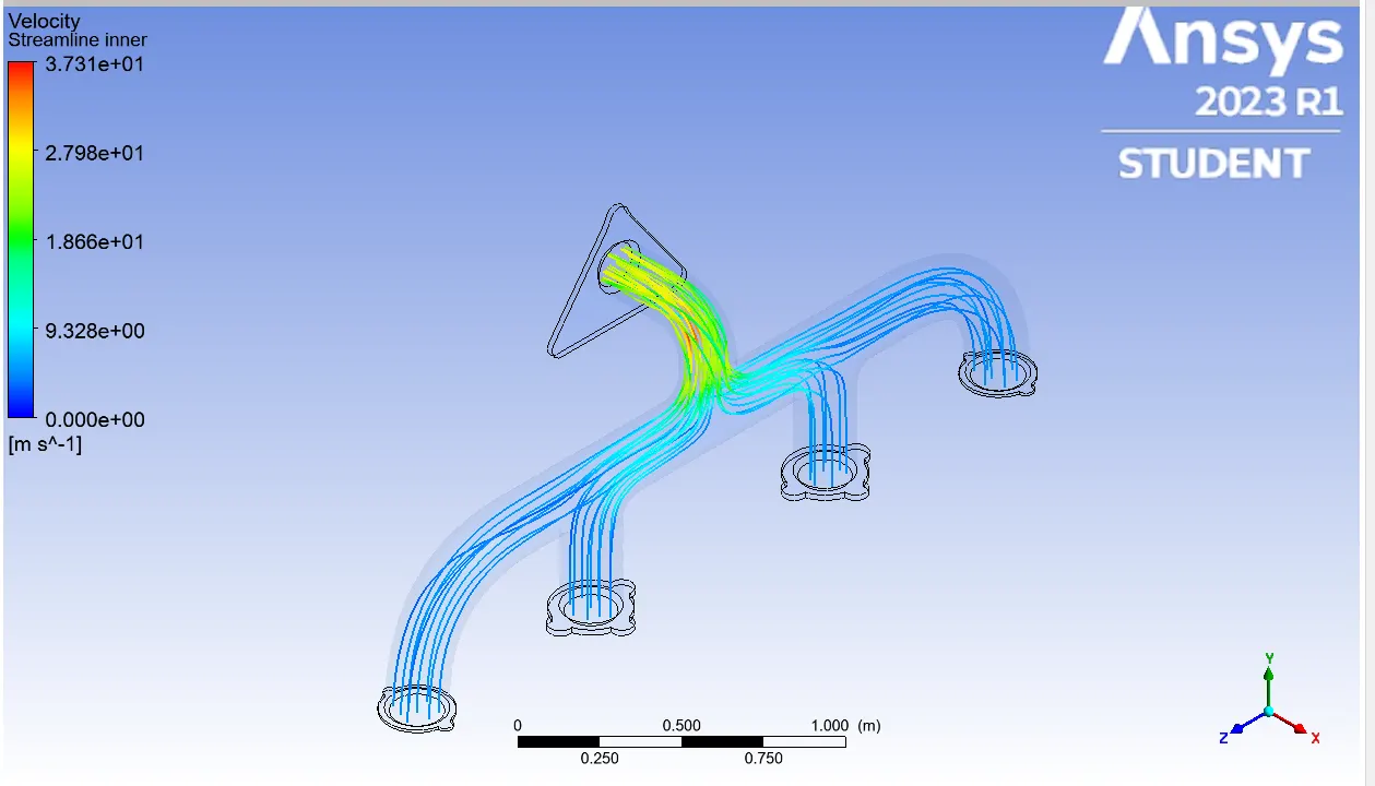
B. Highest velocity magnitude

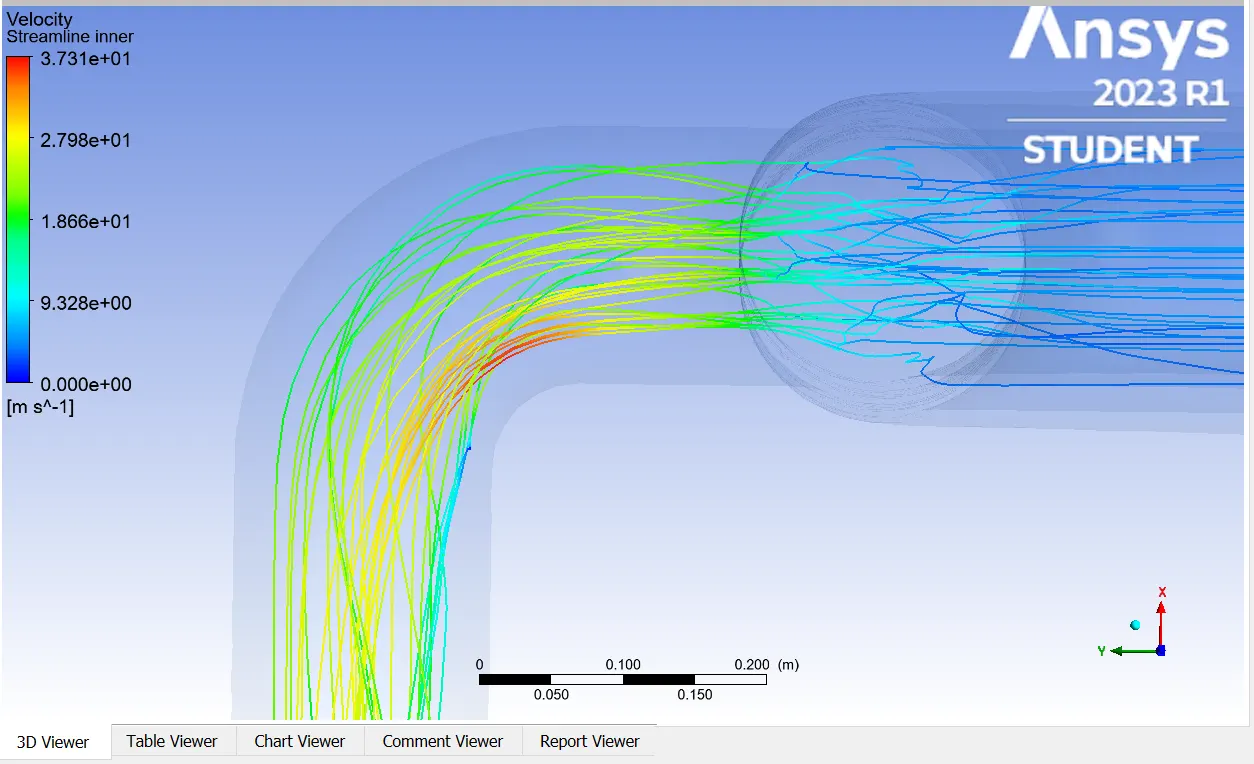
C. General velocity contour at highest velocity magnitude region

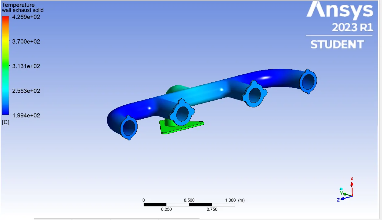
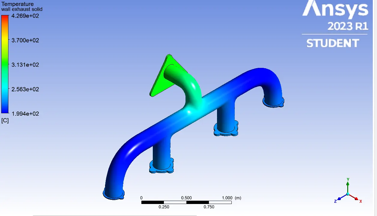
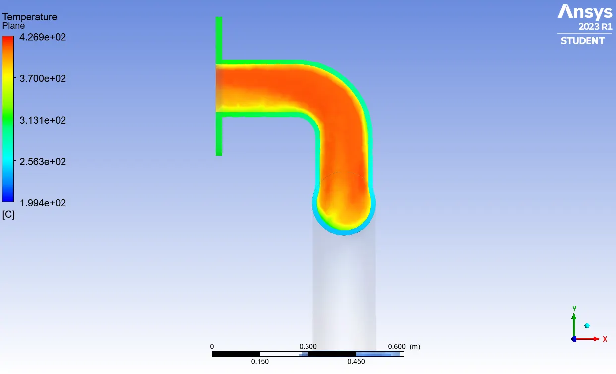
Furthermore, temperature gradient is equal into the exhaust cavity; however, over the exhaust walls the temperature begins to increase due to the heat transfer increment gained by the speed increasing. Then, the following contours show the temperature gradient as inside the exhaust as over the exhaust walls.

• Temperature contours:

A. Temperature gradient on the outer exhaust wall- Isometric bottom view (Inlets)

B. Temperature gradient on the outer exhaust wall- Isometric top view (Main body)

C. Temperature gradient at the critical section of the body

Reviewing the velocity contours shown above and comparing them with the heat transfer contour obtained below, it is clear the heat transfer coefficient will always depend of the flow velocity; looking at the picture where the highest velocity magnitude is shown, it can be then seen the heat transfer coefficient is the highest at the same point too. It must be taken into accoun the velocity increment at that point of the geometry is due to the flow suffer a little shedding because of the streamlines are disturbed by the geometry curves.

• Heat transfer coefficient contours:

A. Heat transfer coefficient at the critial section of the body

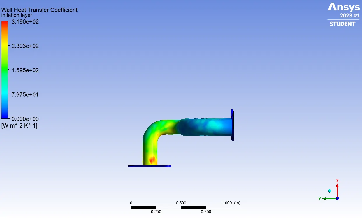
B. Heat transfer coefficient along the body - Bottom view

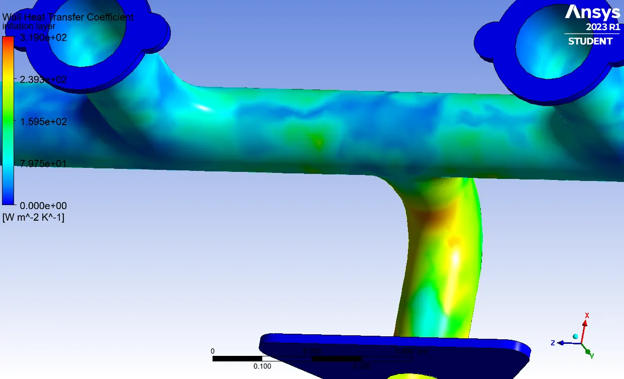
Now, the results obtained by two different experiments only take the inlet pipe diameter, but in this project, it is taken the mean pipe between the inlet and the outlet diameters due to they have not the same measure. So, the results will vary a little because of the reynolds number taken to calculate the wall distance heigth. The results obtained were:

	Turbulence model	Maximum velocity	Maximum HTC
Current project	`k-epsilon`model	37.3 `m/s`	250.7 `W/(m^2K)`
Sharma. U. Project (https://skill-lync.com/student-projects/week-4-cht-analysis-on-exhaust-port-84)	`k-epsilon`model - 2nd refinement	40.4 `m/s`	`258.9 W/(m^2K)`
Misar. P. Project (https://skill-lync.com/student-projects/cht-analysis-on-exhaust-port-8)	`k-omega`model	40.2 `m/s`	`240 W/(m^2K)`

The variation of both results is very important, however, regarding the second project, the mesh size is not refined enough as the first one. The mesh used in this case has 148796 nodes and 375161 elements, that means the accuracy level is good in comparison with the results obtained by the experiment carried out by Sharma. U.

CONCLUSIONS

The CHT correct analysis could be confirmed by comparing the results obtained in other student experiments, likewise, it can also be used other ways to get certainly the results obtained on the simulations are accurate; empirical experiments can be performed and manual calculus are one of these confirmation methods.

Complex geometries become difficult the way to take the real characteristic length; it is adviced by different researches to get the volume and superficial object area, using CAD programs, and divide the volume obtained over the superficial object area. This advisement is only for objects that are exposed to external flows.

REFERENCES

https://forum.ansys.com/forums/topic/difference-between-k-epsilon-and-k-omega-turbulence-model/

https://lms.skill-lync.com/programs/94933/23/choosing-a-right-turbulence-model/knowledgebase

https://skill-lync.com/student-projects/week-4-cht-analysis-on-exhaust-port-84 - Paper results from 1st student

https://skill-lync.com/student-projects/cht-analysis-on-exhaust-port-8 - Paper results from 2nd student

https://www.simscale.com/docs/analysis-types/conjugate-heat-transfer-analysis/