Project 2 - Rankine cycle Simulator

• Project 2- Rankine Cycle Simulator code:

%Rankine Cycle Simulator 
%Diego Alejandro Cepeda Cuartas

close all
clear all
clc

%The following code sheet will help calculating the all cycle rankine entered by an user. When the user enters turbine inlet pressure and temperature and, the turbine outlet pressure, the program will calculate the all rankine cycle. 
% 1. Rankine Cycle Explanation
% 1-2 Isentropic expanssion into the turbine 
% 2-3 Heat rejection on the condenser
% 3-4 Isentropic compression on the pump
% 4-1 Heat addition to constant pressure into the boiler
disp("                      CYCLE RANKING VALUES             ")

%Rankine cycle explanation shown up the screen 
disp("1-2 Isentropic expanssion into the turbine") 
disp("2-3 Heat rejection on the condensator")
disp("3-4 Isentropic compression on the pump")
disp("4-1 Heat addition to constant pressure into the boiler")

% 2. Defining inputs required 
a=input('Select the turbine inlet pressure in bar: ','s');
P1=str2double(a);
b=input('Now, select the turbine inlet temperature in °C: ','s');
T1=str2double(b);
c=input('Finally, select the turbine outlet pressure in bar: ','s');
P2=str2double(c);

% 3. Calling the Xsteam function to calculate the enthalpy and entropy

%Saturated Gas 
h1=XSteam('h_pt',P1,T1); % Turbine Inlet Enthalpy
s1=XSteam('s_pt',P1,T1); %Turbine Inlet Entropy

%S1=S2 because the expansion is carried out in a isentropic way
s2=s1;% Condenser Inlet Entropy 
hf2=XSteam('hL_p',P2);
hg2=XSteam('hV_p',P2);
sf2=XSteam('sL_p',P2);
sg2=XSteam('sV_p',P2);
x2=((s2-sf2)/(sg2-sf2));%Vapor quality 
h2=hf2+(x2*(hg2-hf2)); % Condenser Inlet Enthalpy
T2=XSteam('T_ph',P2,h2);
Tsat2=XSteam('Tsat_p',P2);

%Saturated Liquid
h3=hf2; %Pump Inlet Enthalpy 
s3=sf2; %Pump Inlet Entropy
v3=XSteam('vL_p',P2);% Specific volume from pump 
P3=P2; %Pump Inlet Pressure
T3=XSteam('Tsat_p',P2);

P4=P1; % Boiler Inlet Pressure  
Wb=v3*(P4-P3)*100; %1bar = 100kPa
h4=h3+Wb; %Boiler Inlet Enthalpy 
s4=s3; %Boiler Inlet Entropy
cp4=XSteam('Cp_ps',P4,s4);%Specific heat at constant pressure
cv4=XSteam('Cv_ps',P4,s4);%Specific heat at constant volume
gamma=cp4/cv4;%Adiabatic gas constant
T4=T3*(P4/P3)^((gamma-1)/gamma);

%Pump and Turbine Power
Wp=Wb ;%Pump
Wt=h1-h2 ;%Turbine

%Boiler and Condenser heat 
Qin=h1-h4; %Boiler 
Qout=h2-h3; %Condenser 

%Net Power
Wnet=Qin-Qout;
Wneto=Wt-Wp;

%Thermal efficiency 
Nther=100*(1-(Qout/Qin));

%Specific Steam Consumption
SSC=3600/(Wnet);

% 4. Plotting both charts (H-s) & (T-s)
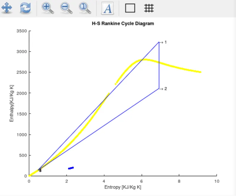
%H-s
T=linspace(0,1.5*T1,800);
figure(1)
hold on 
for i=1:length(T)
  plot(XSteam('sL_T',T(i)),XSteam('hL_T',T(i)),'.','color','y');
  plot(XSteam('sV_T',T(i)),XSteam('hV_T',T(i)),'.','color','y');
end
;
plot([s1 s2],[h1 h2],'color','b')
plot([s2 s3],[h2 h3],'color','b')
plot([s3 s4],[h3 h4],'color','b')
plot([s4 s1],[h4 h1],'color','b')

text(s1,h1,'\rightarrow 1')
text(s2,h2,'\rightarrow 2')
text(s3,h3,' 3')
text(s4,h4,' 4')
xlabel('Entropy [KJ/Kg K]')
ylabel('Enthalpy[KJ/Kg K]')
title('H-S Rankine Cycle Diagram')

%T-s
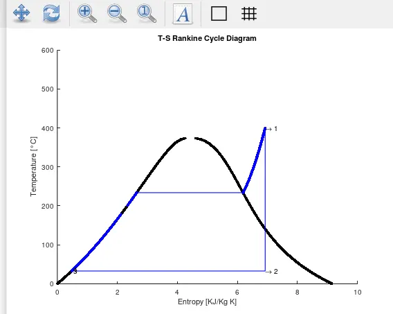
figure(2)
hold on 

for i=1:length(T)
  plot(XSteam('sL_T',T(i)),T(i),'.','color','k');
  plot(XSteam('sV_T',T(i)),T(i),'.','color','k');
end
;
plot([s1 s2],[T1 T2],'color','b')
if (x2>1)
  T3=Tsat2
  plot([s2 sg2 s3 s4],[T2 Tsat2 T3 T4],'color','b')
  T2=Tsat2
else
  plot([s2 s3 s4],[T2 T3 T4],'color','b')
end 
;
Te=linspace(T1,T2,800);
for i=1:length(Te)
  plot(XSteam('S_pT',P1,Te(i)),Te(i),'color','b');
end
;

plot([XSteam('sL_p',P1) XSteam('sV_p',P1)],[XSteam('Tsat_p',P1) XSteam('Tsat_p',P1)],'color','b')
text(s1,T1,'\rightarrow 1')
text(s2,T2,'\rightarrow 2')
text(s3,T3,' 3')
text(s4,T4,' 4')
xlabel('Entropy [KJ/Kg K]')
ylabel('Temperature [°C]')
title('T-S Rankine Cycle Diagram')

% 5. Showing the values 
disp("                           RESULTS                     ")
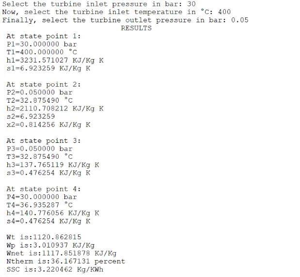
fprintf(' At state point 1:\n P1=%f bar \n T1=%f °C\n h1=%f KJ/Kg K\n s1=%f KJ/Kg K\n',P1,T1,h1,s1) 
fprintf('\n At state point 2:\n P2=%f bar \n T2=%f °C\n h2=%f KJ/Kg K\n s2=%f\n x2=%f KJ/Kg K\n',P2,T2,h2,s2,x2) 
fprintf('\n At state point 3:\n P3=%f bar \n T3=%f °C\n h3=%f KJ/Kg K\n s3=%f KJ/Kg K\n',P3,T3,h3,s3) 
fprintf('\n At state point 4:\n P4=%f bar \n T4=%f °C\n h4=%f KJ/Kg K\n s4=%f KJ/Kg K\n',P4,T4,h4,s4)
fprintf('\n Wt is:%f\n Wp is:%f KJ/Kg \n Wnet is:%f KJ/Kg \n Ntherm is:%f percent \n SSC is:%f Kg/KWh',Wt,Wp,Wnet,Nther,SSC)

• Diagrams obtained:
• T-s Diagram

• H-s Diagram

• Results

• Results required:
• Net work output:

Wnet=1117.852 KJ/ Kg K

• Back work ratio:

Nb= Wp/Wt= 0.002686

• Google Drive report link:

https://docs.google.com/document/d/1FnXtAPvbj18jv0SlAOFtWizqKWvI0fQiEbfRtbIJNYc/edit?usp=sharing