Week 7 - Simulation of a 1D Super-sonic nozzle flow simulation using Macormack Method
Problem Statement:
1. To derive the conservation and non-conservation form for the subsonic supersonic flow through the nozzle using Mac-Cormack's technique.
2. To simulate the subsonic and supersonic flow through the nozzle and using both conservative and non-conservative form.
3. To determine the steady-state temperature distribution of flow field variables.
4. To study the difference between the conservative and non-conservative form of governing equations.
Introduction:
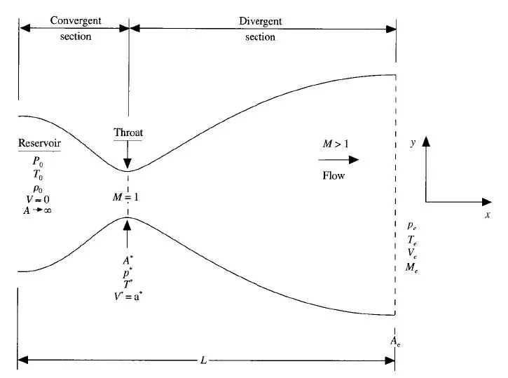
In the flow consider, the nozzle is a convergent-divergent nozzle where the convergent part of the nozzle is attached to the reservoir which has stagnant pressure and temperature. The flow through the nozzle is isentropic flow. The area of the convergent nozzle is large hence the initial velocity is low and at the throat of the nozzle, the flow is sonic where Mach number(M) =1 and with increasing the area the velocity increases at this stage the flow breaks the sound barrier and attains supersonic speed where Mach number>1.
Assumption:
We assume that the flow variables are varying in x-direction ie., along the length of the nozzle. This is done to assume uniform flow properties across the cross-section of the nozzle. This type of flow is called quasi-one-dimensional flow.
Approach:
1. The Governing equations will be written in terms of the partial differential equations suitable for time marching solution for quasi 1D flow.
2. The finite difference model using the Mac Cormack technique is applied to the problem given.
3. Time step size, courant number, and initial and boundary conditions are formulated.
4. Use of the initial conditions to obtain approximate the converge flow variables for the next time step till a steady state is achieved.
Mac Cormack's Method:
In CFD, MacCormack's technique is widely used in the discretization scheme for parabolic partial differential equations. The PDE is of second order.
The MacCormack technique proceeds in two steps i.e., the predictor step followed by the corrector step.
In the predictor step, the gradient value of the governing equation at time step n is estimated with known values at time step n. In this step forward differencing scheme is used.
Then flow variables are calculated at time step n+1 with known values of flow variable at time step n along with gradient.
In the corrector step, the values of the gradient at time step n+1 is estimated with the known values at time step n+1 i .e., obtained from the predicted step. In this step backward differencing scheme is used.
The average of the gradients of the predicted step and corrector step is calculated.
Then flow variables at the n+1 time step are calculated using flow variables at time step n and average gradients are calculated.
Governing Equations:
Continuity Equation:
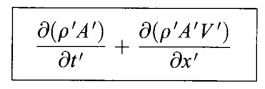
Momentum Equation:
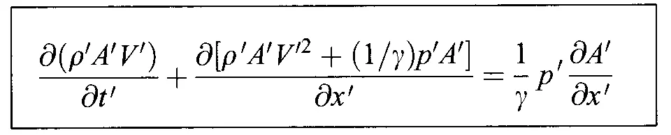
Energy equation :

Governing Equations in Non-Conservative Form
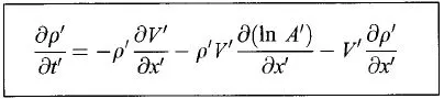
Continuity Equation:
Momentum Equation:
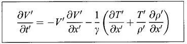
Energy Equation:

In the above equation (') on the flow variables represent that they are non-dimensionalized.
V' - velocity
T' - temperature
`rho'` is density
A' is the area of the nozzle for the length x.
Discretization of the above governing equations:
`((delrho)/dt)_i^t = -rho_i^t*(V_(i+1)^t-V_(i)^t)/dx-rho_(i)^t*V_(i)^t*(ln(A_(i+1))-ln(A_(i)))/dx-V_(i)^t*(rho_(i+1)^t-rho_(i)^t)/dx`
`((delV)/(delt))_i^t= -V_i^t * (V_(i+1)^t-V_i^t)/dx+(1/gamma)*((T_(i+1)^t-T_i^t)/dx+T_i^t/rho_i^t*(rho_(i+1)^t-rho_i^t)/dx)`
`((delT)/(delt))_i^t = -V_i^t*(T_(i+1)-T_i^t)/dx-(gamma-1)*T_i^t*((V_(i+1)^t-V_i^t)/dx+V_i^t*(lnA_(i+1)-lnA_i)/dx)`
Discretizing the time derivative term
`(rho)_i^(t+trianglet) = (rho)_i^t+((delrho)/(delt))_i^t*trianglet`
`(V)_i^(t+trianglet) = (V)_i^t+((delV)/(delt))_i^t*trianglet`
`(T)_i^(t+trianglet) = (T)_i^t+((delT)/(delt))_i^t*trianglet`
`(T)_i^(t+trianglet)`, `(V)_i^(t+trianglet)` , `(rho)_i^(t+trianglet)` are the predicted values
`(T)_i^t `,`(V)_i^t `,`(rho)_i^t` are known values at time t
Corrector Step:
`((delrho)/dt)_i^(t+trianglet) = -rho_i^(t+trianglet)*(V_(i)^(t+trianglet)-V_(i-1)^(t+trianglet))/dx-rho_(i)^(t+trianglet)*V_(i)^(t+trianglet)*(ln(A_(i))-ln(A_(i-1)))/dx-V_(i)^(t+trianglet)*(rho_(i)^t-rho_(j-1)^t)/dx`
`((delV)/(delt))_i^(t+trianglet)= -V_i^(t+trianglet) * (V_(i)^(t+trianglet)-V_(i-1)^(t+trianglet))/dx+(1/gamma)*((T_(i)^(t+trianglet)-T_(i-1)^(t+trianglet))/dx+T_i^(t+trianglet)/rho_i^(t+trianglet)*(rho_(i)^(t+trianglet)-rho_(i-1)^(t+trianglet))/dx)`
`((delT)/(delt))_i^(t+trianglet) = -V_i^(t+trianglet)*(T_(i)^(t+trianglet)-T_(i-1)^(t+trianglet))/dx-(gamma-1)*T_i^(t+trianglet)*((V_(i)^(t+trianglet)-V_(i-1)^(t+trianglet))/dx+V_i^(t+trianglet)*(lnA_(i)-lnA_(i-1))/dx)`
Calculating the average of the slopes from predicted and corrector step
`((delrho)/(delt))_(avg) = 0.5 [((delrho)/(delt))_i^t+((delrho)/(delt))_i^(t+trianglet) ]`
`((delV)/(delt))_(avg) = 0.5 [((delV)/(delt))_i^t+((delV)/(delt))_i^(t+trianglet) ]`
`((delT)/(delt))_(avg) = 0.5 [((delT)/(delt))_i^t+((delT)/(delt))_i^(t+trianglet) ]`
Calculating the approximated values with the average of slopes calculated above:
`(rho)_i^(t+trianglet) = (rho)_i^t+((delrho)/(delt))_(avg)*trianglet`
`(V)_i^(t+trianglet) = (V)_i^t+((delV)/(delt))_(avg)*trianglet`
`(T)_i^(t+trianglet) = (T)_i^t+((delT)/(delt))_(avg)*trianglet`
`(T)_i^(t+trianglet)`, `(V)_i^(t+trianglet)` , `(rho)_i^(t+trianglet)` are the final approximated values for the time step `t+trianglet`
`(T)_i^t `,`(V)_i^t `,`(rho)_i^t` are known values at time t
where `trianglet= C*((trianglex)/(a+V))`
C is the courant Number which is equal to 0.5.
`trianglex` is the grid spacing
a is speed of sound
`a = sqrt(T)`
V is velocity of the flow.
In the calculation of the time step there are two ways:
1. Finding the local values of `(trianglet)_i^t` for each grid point. As the flow is advancing the flow variables are calculated at each grid point at their own time step. This method leads to a faster convergence rate to the steady-state. This method is also chosen if the final steady-state is the desired output result.
2. The other method is to calculate `(trianglet)_i^t` at all grid points and then choose the minimum value. The resulting value is used in the above-discretized equation. This solution gives a time-accurate solution for the transient flow field consistent with the unsteady continuity, momentum, and energy equations.
The second method is used to solve the non-conservation and conservation form.
Boundary Conditions:
Boundary conditions are an important aspect of solving governing equations because without proper implementation of the boundary conditions we cannot find the solutions to any flow problem.
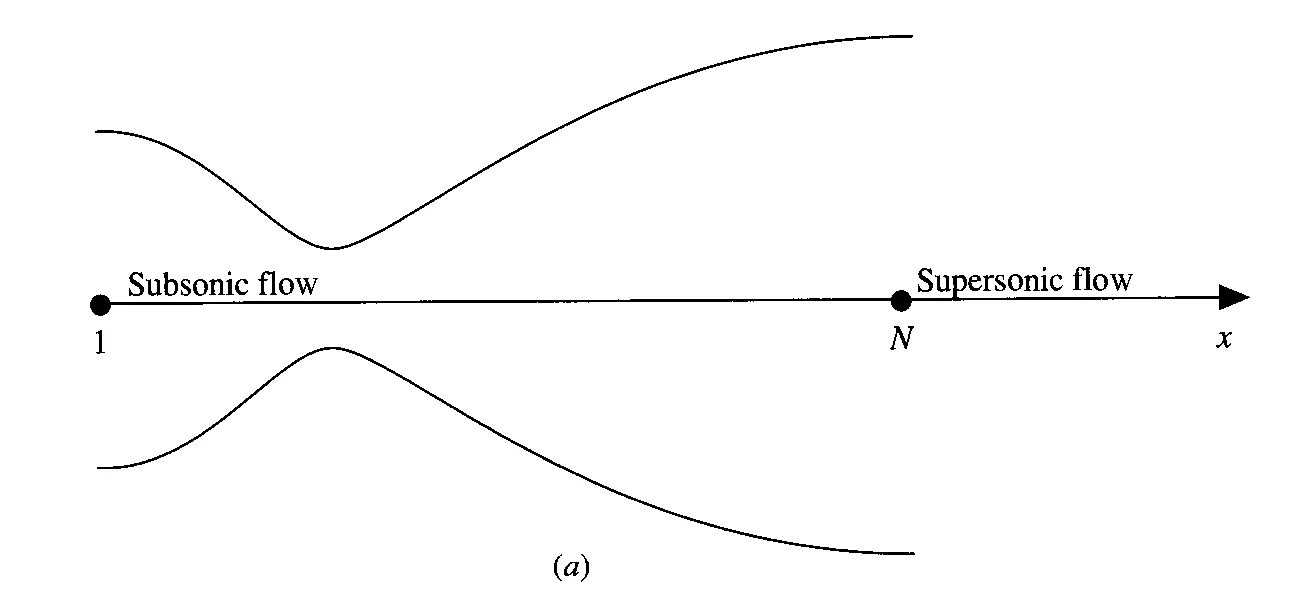
In the figure given above grid point 1 represents subsonic flow and grid point N represent the supersonic flow. At grid point 1 represents the inflow boundary point where the area is finite. If the area is infinite then the velocity will be equal to zero and there will no mass flow rate hence the area is considered finite in solving the 1D subsonic supersonic nozzle flow.
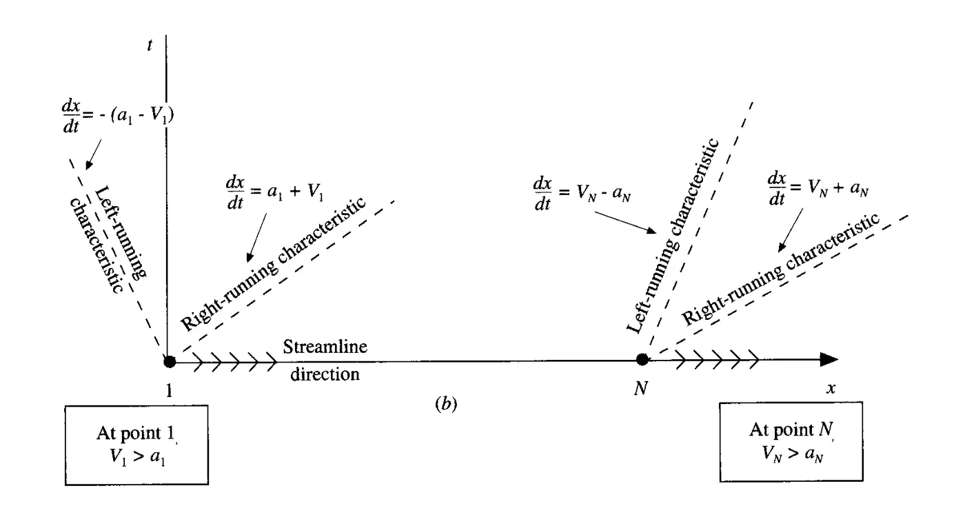
The flow considered is an unsteady inviscid flow which is governed by hyperbolic equations and there exist two characteristics lines i.e., left running characteristics line and right running characteristics line for grid points 1 and N as shown in the figure. The characteristics line represents weak Mach number wave running left and right relative to the flow with velocity '(a-V)' and '(a+V)' respectively. In grid point 1 the wave is traveling upstream with velocity `(a_1-V_1)` represented by left running characteristics line against low subsonic wave which is traveling from left to right. Since the domain is from the grid point 1 to N. The left running characteristics line is out of the domain whereas the right running characteristics line is inside the domain. This is because the flow is running already running from left to right and the right running characteristics are moving towards the right with a velocity of sound 'a' relative to the flow, hence the right running characteristics are moving with the combined velocity of (`V_1+a_1`).
From the above method of characteristics, we can infer that when one characteristics line runs out of the domain then one dependent variable should be specified in the boundary and if the characteristics line is within the domain then another dependent variable is allowed to float that is it must be specified at all time step as a function of time-wise solution to the flow field. At the subsonic inflow boundary, we must fix the values of two dependent variables and allow one dependent variable to float.
In the same way boundary conditions for grid point N can be analyzed were both left running characteristics line and right running characteristics line is running outside the domain hence all the dependent variables must be allowed to float.
In Subsonic Inflow boundary we consider velocity to float and pressure and temperature to be fixed as the pressure and temperature are stagnant at the reservoir and very low and velocity is rapidly changing with the area and another reason is the mass flow through the nozzle adjust itself to attain steady state. Hence it is desirable to choose velocity to float at the inflow boundary condition. The velocity at grid point 1 is calculated with inner grid points using linear extrapolation.
`V_1 = 2*V_2-V_3`
`rho_1 =1` `
`T_1 = 1`
here density and temperature are fixed independent of time.
In Supersonic outflow boundary since all the dependent variables are allowed to float boundary conditions for density (`rho`), temperature(T), velocity(V) is specified at the outlet boundary conditions
`V_N = 2*V_(N-1)-V_(N-2)`
`(rho)_N = 2*(rho)_(N-1)-(rho)_(N-2)`
`T_N = 2*T_(N-1)-T_(N-2)`
Nozzle shape: Since the nozzle is a convergent-divergent nozzle we choose the parabolic area distribution which is given as
`A = 1+2.2*(x-1.5)^0.5` where `0<=x<=3`
At x=1.5 A represents the throat area and `0<=x<=1.5` represents the convergent part of the nozzle and `1.5<=x<=3` represents the divergent part of the nozzle.
Initial Conditions:
Initial Conditions should be selected wisely because closer the value initial conditions to the final steady-state values faster the convergence rate.
If the initial conditions are chosen far away from the steady-state solution the initial time-wise gradients at early time steps will be large. For the given time step `trianglet` and spacial dimension, `trianglex` gradients obtained are large for early time steps which leads to unstable solutions. As time progresses the flow field approaches a steady-state and hence slowing down the rate of approach.
In the present problem, we know that pressure and temperature decrease, and velocity increases in the direction of flow, and hence the following equations are chosen.
`rho = 1-0.3146*x`
`T = 1-0.2314*x`
`V = (0.1+1.09*x)*T^0.5`
The values for `rho , V, T` are initial conditions at t = 0.
Conservative Form:
The governing equation in conservation form represents the actual physics of the flow. Hence there will no change in the governing equations mentioned above.
There are
Continuity Equation:
Momentum Equation:
Energy equation :
In the above equation (') on the flow variables represent that they are non dimensionalized.
V' - velocity
e' = T'
T' - temperature
`rho'` is the density
A' is the area of the nozzle for the length x.
From the above quasi 1D flow equation the flow variables are represented in terms solution vector U, flux vector F and source term J
To reduce the complexity of the equation (') is avoided
`U_1 = rho*A`
`U_2 = rho*A*V`
`U_3 = rho*(T/(gamma-1)+gamma/2*V^2)*A`
`F_1 = rho*A*V`
`F_2 = rho*A*V^2+1/gamma*rho*A`
`F_3 = rho*(T/(gamma-1)+gamma/2*V^2)*V*A+rho*A*V`
`J_2 = 1/gamma*rho*(delA)/(delx)`
Governing equations in terms of the U,F and J are
`(delU_1)/(delt) = -(delF_1)/(delx)`
`(delU_2)/(delt) = -(delF_2)/(delx)+J_2`
`(delU_3)/(delt) = -(delF_3)/(delx)`
The above governing equations are solved numerically using Mac Cormack technique. It is to be noted that in the above governing equations the dependent variables are in terms of U not the primitive variables. Mac Cormack technique gives converged values of U from which flow variables can be calculated.
`rho = U_1/A`
`V = U_2/U_1`
`T = (gamma-1)*(U_3/U_1-gamma/2*V^2)`
`P = rho*T`
When flux variables are written in terms of flow variables instability develop over the time marching process. This is because of lack of purity of the numerical formulation of the governing equations in conservation form. Hence flux variables are written interms of solution variables inorder to have purity of the governing equations in terms of solution variables.
`F_1 = U_2`
`F_2 = U_2^2/U_1+(gamma-1)/gamma*(U_3-gamma/2*U_2^2/U_1)`
`F_3=gamma*(U_2*U_3)/U_1-(gamma*(gamma-1))/2*U_2^3/U_1^2`
`J_2=(gamma-1)/gamma*(U_3-gamma/2*U_2^2/U_1)*(del(lnA))/(delx)`
Boundary Conditions:
Boundary conditions for the conservative form are the same as the non-conservative form where at the inflow boundary one dependent variable is allowed to float and two dependent variables are fixed and at the outflow boundary, all the flow variables are allowed to float.
At the inflow boundary `rho, T`are fixed and V is allowed to float and at the outflow `rho, T and V` are allowed to float.
The above boundary conditions written in terms of solution variables U for inflow boundary is given by
`U_1= rho_1*A_1` where `rho`is fixed at the inflow and area is constant which results in
`U_1 = fixed`
`U_2 = 2*U_2^2-U_2^3` where superscript represents the grid positions.
`U_3 = U_1*(T/(gamma-1)+gamma/2*V^2)`
The value of `U_3` is found at the 1st grid point. where T and V values are also 1st grid point.
The boundary conditions for the outflow boundary is given by
`(U_1)_N = 2*(U_1)_(N-1)-(U_1)_(N-2)`
`(U_2)_N = 2*(U_2)_(N-1)-(U_2)_(N-2)`
`(U_3)_N = 2*(U_3)_(N-1)-(U_3)_(N-2)`
Initial Conditions:
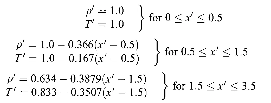
Initial conditions entered for conservative form slightly realistic than those assumed in non-conservative form. This is done because the discretization form of the conservative form of governing equations is more sensitive and it is useful to start with improved initial conditions.
The Timestep calculation for the conservative form is the same as the non-conservative form. As both equations are hyperbolic in nature for an explicit equation the stability criteria are governed by the CFL condition with which the `trianglet` is calculated.
Matlab code is written to solve the governing equations of Conservative and non-Conservative form using Mac-Cormack's Technique.
Main Script
%Code to Plot the steady state and time wise variation of the flow
%variables of the subsonic supersonic flow through the nozzle and to
%compare the mass flow rate in conservation and non conservation form.
close all
clear all
clc

%Specifing the number of grid points

n = 31;

%Calling for the function to calculate the flow variables of the non
%conservative form of subsonic supersonic flow through a nozzle.

[mass_nc,rho_nc,t_nc,p_nc,v_nc,a_nc,M_nc] = non_conservative(n);

%Calling for the function to calculate the flow variables of the
%conservative form of subsonic supersonic flow through a nozzle.

[x,mass_c,rho_c,t_c,P_c,v_c,M_c] = conservative(n);

%Plot showing the comparison of mass flow rate of the both forms
figure(6)
plot (x,mass_nc)
hold on
plot (x,mass_c)
title('Comparison of the mass flow rate of conservative and non conservative form at steady state')
xlabel('length of the nozzle')
ylabel('non dimensional mass flow rate')
legend('Non conservative form','Conservative form')
Explanation of the Main script:
1. Defining the number of grid points.
2. Call of the function to calculate the flow variables of the non-conservative form of subsonic supersonic flow through a nozzle that takes an input number of grid points and outputs flow variables.
3. Call of the function to calculate the flow variables of the conservative form of subsonic supersonic flow through a nozzle that takes an input number of grid points and outputs flow variables.
4. Plotting of the graph which compares the mass flow rate of conservative and non-conservative form.
Function to calculate the flow variables of the non-conservative form of subsonic supersonic flow through a nozzle.
%Calling for the function to calculate the flow variables of the non
%conservative form of subsonic supersonic flow through a nozzle.

function [mass,rho,t,P,v,a,M] = non_conservative(n)

    %inputs for the non conservation equations
    x = linspace(0,3,n);%<-- specifing the values of the position of grid points
    dx = x(2)-x(1);%<-- Calculating the grid spacing


    %Input Boundary conditions
    rho = 1-0.3146*x;
    t = 1-0.2314*x;
    v = (0.1+1.09*x).*t.^0.5;
    a = 1+2.2*(x-1.5).^2;


    gamma = 1.4;%<-- heat capacity ratio
    throat = find(a==1);%<-- Finding the position of throat where area =1.


    %Calculation of time step size.
    c=0.5;%<-- CFL criteria
    s= sqrt(t);
    dt =min(c*dx./(s+v));

    %Defining the number of time steps
    nt = 1400;

    %  time loop
for h = 1:nt

    %Storing the previous iteration time step converged values.
        vold = v;
        rhoold=rho;
        told = t;

   %For loop to calculate the flow variables in the predictor step
        for j = 2:n-1

        % Inorder to reduce the complexity of the governing equations below
        %terms are repeatative and calculated first and then later entered
        %into the governing equations.
        dvdx = (v(j+1)-v(j))/dx;
        dlogadx = (log(a(j+1))-log(a(j)))/dx;
        drhodx = (rho(j+1)-rho(j))/dx;
        dtdx = (t(j+1)-t(j))/dx;

         %Predicted values calculation.
        drhodt_p(j) = -rho(j)*dvdx-rho(j)*v(j)*dlogadx-v(j)*drhodx;
        dvdt_p(j) = -v(j)*dvdx-(1/gamma)*(dtdx+(t(j)/rho(j))*drhodx);
        dtdt_p(j) = -v(j)*dtdx-(gamma-1)*t(j)*(dvdx+v(j)*dlogadx);

        %Updating the flow variables with the predicted gradients calculated
        rho(j) = rho(j)+drhodt_p(j)*dt;
        v(j) = v(j)+dvdt_p(j)*dt;
        t(j) = t(j)+dtdt_p(j)*dt;


        end

%Corrector step
%For loop to calculate the flow variables with the predicted flow variables

    for jj = 2:n-1

         %Corrected values calculation.

        dvdx = (v(jj)-v(jj-1))/dx;
        dlogadx = (log(a(jj))-log(a(jj-1)))/dx;
        drhodx = (rho(jj)-rho(jj-1))/dx;
        dtdx = (t(jj)-t(jj-1))/dx;

        drhodt_c(jj) = -rho(jj)*dvdx-rho(jj)*v(jj)*dlogadx-v(jj)*drhodx;
        dvdt_c(jj) = -v(jj)*dvdx-(1/gamma)*(dtdx+(t(jj)/rho(jj))*drhodx);
        dtdt_c(jj) = -v(jj)*dtdx-(gamma-1)*t(jj)*(dvdx+v(jj)*dlogadx);


    end

      %Taking the average of the gradients of the predicted and corrector
      %step
      drhodt_avg = 0.5*(drhodt_p+drhodt_c);
      dvdt_avg = 0.5*(dvdt_p+dvdt_c);
      dtdt_avg = 0.5*(dtdt_p+dtdt_c);

      %For loop to calculate the final update solution using the average
      %gradients
      for ii = 2:n-1

      rho(ii) = rhoold(ii) + drhodt_avg(ii)*dt;

      v(ii) = vold(ii)+dvdt_avg(ii)*dt;

      t(ii) = told(ii)+dtdt_avg(ii)*dt;

      end


     %Defining initial boundary conditions
      v(1) = 2*v(2)-v(3);

     %Defining outflow Boundary conditions
      rho(n) = 2*rho(n-1)-rho(n-2);
      v(n) = 2*v(n-1)-v(n-2);
      t(n) = 2*t(n-1)-t(n-2);

      %Calculation of flow variable at throat where area(a)=1
      rho_t(h) = rho(throat);%<-- density at throat
      t_t(h) = t(throat);%<-- Temperature at throat
      v_t(h) = v(throat);%<-- velocity at throat
      P_t(h) = rho(throat).*t(throat);%<-- Pressure at throat
      M_t(h) = v(throat)./sqrt(t(throat));%<-- Mach number at throat
      mass = rho.*v.*a;

      %if else condition to plot the variation of non dimensional mass flow
      %rate at specific time steps and plot the same
       if h == 50
          %plotting of mass flow rate at time step 50
          figure(7)
          plot(x,mass)
          hold on
      elseif h == 100
          %plotting of mass flow rate at time step 100
          plot (x,mass)
      elseif h==150
          %plotting of mass flow rate at time step 150
          plot(x,mass)
       elseif h==200
           %plotting of mass flow rate at time step 200
           plot (x,mass)
       elseif h==700
           %plotting of mass flow rate at time step 700
           plot (x,mass)
           title ('Plot of mass flow rate at different time steps Non conservative form')
           xlabel('Nozzle length')
           ylabel('Non-dimensional Mass flow rate')
           legend ('50','100','150','200','700')
       end


end

%Calculation of mach number for the steady state
M = v./sqrt(t);
%Calculation of pressure for the steady state.
P = rho.*t;
%Calculation of mass flow rate for the steady state.
mass = rho.*v.*a;

%Plot for Steady State variation of converged primitive variables inside nozzle
figure(1)

    subplot(5,1,1)
    plot(x,v)
    title('Time step:',h)
    xlabel('length of nozzle')
    ylabel('velcoity')


     subplot(5,1,2)
    plot(x,t)
    title('Time step:',h)
    xlabel('length of nozzle')
    ylabel('Temperature')


    subplot(5,1,3)
    plot(x,rho)
    title('Time step:',h)
    xlabel('length of nozzle')
    ylabel('Density')


    subplot(5,1,4)
    plot(x,M)
    title('Time step:',h)
    xlabel('length of nozzle')
    ylabel('Mach number')


    subplot(5,1,5)
    plot(x,P)
    title('Time step:',h)
    xlabel('length of nozzle')
    ylabel('Pressure')
    sgtitle('Steady state of primitive variables for non conservative form')


   %time wise variation of flow variables at throat for each time step.
    figure(2)

    subplot(4,1,1)
    plot(t_t)
    xlabel('time step')
    ylabel('Temperature')


    subplot(4,1,2)
    plot(rho_t)
    xlabel('time step')
    ylabel('Density')


    subplot(4,1,3)
    plot(M_t)
    xlabel('time step')
    ylabel('Mach number')


    subplot(4,1,4)
    plot(P_t)
    xlabel('time step')
    ylabel('Pressure')
    sgtitle('Time wise variation of primitive variables for non conservative form')


end
Explanation of the above function used for non-conservation form:
1. Function takes the number of grid points(n) as input.
2. With n, the position of the grid points is obtained and grid spacing is calculated.
3. With the position of the grid points are known the initial boundary conditions for the flow variables are calculated.
4. Heat capacity ratio is defined and throat position is found using find command with condition a==1.
5. The governing equation of non-conservative form is of explicit form which is governed by stability criteria where CFL =0.5 with which the time step size is calculated.
6. Time loop is created to calculate the steady-state flow variables. No. of the time loop is of 1400.
7. Inside the time loop, a copy of the previous iteration time step value is made which is later used in the final update of the solution.
8. For the calculation of the predicted values for each time step a for loop is created. The for loop is between the 2nd grid point to the 30th grid point since the initial and last boundary values are defined in boundary conditions.
Flow variables are updated using the predicted step derived above for non-conservative form inside the predictor for loop.
9. Another for loop is created to calculate the gradients for the corrector step using the equation derived for non-conservative form.
10. Then the average of the predictor and corrector gradients are calculated.
11. Another for loop is created for the final update of the flow variables with the gradient average.
12. Inflow and outflow boundary conditions are defined. The reason for defining them at the end of the calculation is that the value of the boundaries depends on the converged values of the inner grid points. Hence the boundary conditions for the flow variables are defined at the end.
13. Storing the values of the flow variables at the throat section to plot the time-wise variation of the flow variables at the throat.
14. If else statements are created to plot the mass flow rate at different time steps to study the variation of the mass flow rate at different time steps till it reaches the steady-state.
15. Mach number(M_nc), pressure(P_nc) and mass flow rate(mass_nc) is calculated.
16. Two plots are created one for steady-state distribution of the flow variables for the length of the nozzle and time-wise variation of the flow variables for the number of time steps.
Function to calculate the flow variables of the conservative form of subsonic supersonic flow through the nozzle.
%Calling for the function to calculate the flow variables of the
%conservative form of subsonic supersonic flow through a nozzle.

function [x,u2,rho,t,P,v,M] = conservative(n)

%inputs
x = linspace(0,3,n);%<-- specifing the values of the position of grid points
dx=x(2)-x(1);%<-- Calculating the grid spacing
a=1+2.2*(x-1.5).^2;%<-- Defining the area of the convergent divergent nozzle
gamma = 1.4; %<-- heat capacity ratio

%defining the initial conditions

for i = 1:n

    if (0<=x(i)&& x(i)<=0.5)
        rho(i) =1;
        t(i) = 1;

    end

    if ((0.5<=x(i)&& x(i)<=1.5))
        rho(i) = 1-0.366*(x(i)-0.5);
        t(i)= 1-0.167*(x(i)-0.5);
    end

    if (1.5<=x(i)&& x(i)<=3)
       rho (i) = 0.634-0.3879*(x(i)-1.5);
       t(i) = 0.833 - 0.3507*(x(i)-1.5);
    end

end

%Initial conditions
v = 0.59./(rho.*a);
u1 = rho.*a;
u2 = 0.59*ones(1,n);
u3 = u1.*((t./(gamma-1))+(gamma/2)*(v.^2));
throat = find(a==1);%<-- Finding the position of throat where area =1.

%time step size calculations
c=0.5;%<-- CFL criteria
s= sqrt(t);
dt =min(c*dx./(s+v));

nt = 1400;%<-- Defining the number of time steps
%  time loop
for h = 1:nt

    %Storing the previous iteration time step converged values.
    u1old = u1;
    u2old = u2;
    u3old = u3;

    %Calculation of flux variables.
    f1 = u2;

    f2 = (u2.^2./u1+(gamma-1)/gamma*(u3-(gamma/2)*u2.^2./u1));

    f3 = ((gamma*u2.*u3)./u1-((gamma*(gamma-1))/2)*(u2.^3)./(u1.^2));

    %for loop to calculate the source term j2
    for i = 1:n-1

    j2(i) = 1/gamma*rho(i)*t(i)*((a(i+1)-a(i))/dx);

    end

    %Predictor Step
    %For loop to calculate the solution variable with flux variable and
    %source term calculated above
    for j= 2:n-1

        du1dt_p(j) = -(f1(j+1) - f1(j))/dx;

        du2dt_p(j) = -(f2(j+1) - f2(j))/dx+j2(j);

        du3dt_p(j) = -(f3(j+1) - f3(j))/dx;

        %Updating the solution variables with the predicted gradients calculated

        u1(j) = u1(j)+ du1dt_p(j)*dt;

        u2(j) = u2(j)+du2dt_p(j)*dt;

        u3(j) = u3(j)+du3dt_p(j)*dt;

    end

    %Calculation of density and temperature to update the previous
    %iteration values which is used in collector step
    rho = u1./a;
    t = (gamma-1)*((u3./u1)-(gamma/2)*(u2./u1).^2);

    %Updating the flux variables with the predicted solution variables.
    f1 = u2;

    f2 = (u2.^2./u1+(gamma-1)/gamma*(u3-(gamma/2)*u2.^2./u1));

    f3 = ((gamma*u2.*u3)./u1-((gamma*(gamma-1))/2)*(u2.^3)./(u1.^2));


%Corrector step
%For loop to calculate the solution variables with the predicted flux
%variables

        for jj = 2:n-1

         du1dt_c(jj) = -(f1(jj) - f1(jj-1))/dx;

        du2dt_c(jj) = -(f2(jj) - f2(jj-1))/dx+(1/gamma)*rho(jj)*t(jj)*(a(jj)-a(jj-1))/dx;

        du3dt_c(jj) = -(f3(jj) - f3(jj-1))/dx;


        end

        %Taking the average of the gradients of the predicted and corrector
        %step
        du1dt_avg = 0.5*(du1dt_c+du1dt_p);
        du2dt_avg = 0.5*(du2dt_c+du2dt_p);
        du3dt_avg = 0.5*(du3dt_c+du3dt_p);

        %For loop to calculate the final update solution using the average
        %gradients
        for k = 2:n-1

            u1(k) = u1old(k)+ du1dt_avg(k)*dt;

            u2(k) = u2old(k)+du2dt_avg(k)*dt;

            u3(k) = u3old(k)+du3dt_avg(k)*dt;

        end

        %Defining initial boundary conditions

        u1(1)=a(1);
        u2(1) = 2*u2(2)-u2(3);
        v(1)=u2(1)/u1(1);
        u3(1) = u1(1)*(t(1)/(gamma-1)+(gamma/2)*v(1)^2);


        %Defining outflow Boundary conditions

        u1(n)=2*u1(n-1)-u1(n-2);

        u2(n)=2*u2(n-1)-u2(n-2);

        u3(n)=2*u3(n-1)-u3(n-2);

        %Calculation of flow variables at each time step
        rho = u1./a;%<-- density calculation

        v = u2./u1;%<--velocity calculation

        t = (gamma-1)*((u3./u1)-(gamma/2)*v.^2);%<-- temperature calculation

      %Calculation of flow variable at throat where area(a)=1
      rho_t(h) = rho(throat);%<-- density at throat
      t_t(h) = t(throat);%<-- Temperature at throat
      v_t(h) = v(throat);%<-- velocity at throat
      P_t(h) = rho(throat).*t(throat); %<-- Pressure at throat
      M_t(h) = v(throat)./sqrt(t(throat));%<-- Mach number at throat

      %if else condition to plot the variation of non dimensional mass flow
      %rate at specific time steps and plot the same
      if h == 100
          %plotting of mass flow rate at time step 100
          figure(5)
          plot(x,u2)
          hold on
      elseif h == 200
          %plotting of mass flow rate at time step 200
          plot (x,u2)
      elseif h==700
          %plotting of mass flow rate at time step 700
          plot(x,u2)
          title ('Plot of mass flow rate at different time steps conservative form')
          xlabel('Nozzle length')
          ylabel('Non-dimensional Mass flow rate')
          legend ('100th time step','200th time step','700th time step')
      end
end

%Calculation of converged flow variables for each time step
rho = u1./a;

v = u2./u1;

t = (gamma-1)*((u3./u1)-(gamma/2)*v.^2);

M = v./sqrt(t);

P = rho.*t;

%Plot for Steady State variation of converged primitive variables inside nozzle
    figure(3)

    subplot(5,1,1)
    plot(x,v)
    title('Time step:',h)
    xlabel('length of nozzle')
    ylabel('Velocity')

    subplot(5,1,2)
    plot(x,t)
    title('Time step:',h)
    xlabel('length of nozzle')
    ylabel('Temperature')

    subplot(5,1,3)
    plot(x,rho)
    title('Time step:',h)
    xlabel('length of nozzle')
    ylabel('Density ')

    subplot(5,1,4)
    plot(x,M)
    title('Time step:',h)
    xlabel('length of nozzle')
    ylabel('Mach number')

    subplot(5,1,5)
    plot(x,P)
    title('Time step:',h)
    xlabel('length of nozzle')
    ylabel('Pressure')
    sgtitle('Steady State of primitive variables for conservative form')


    %time wise variation of flow variables at throat for each time step.
    figure(4)

    subplot(4,1,1)
    plot(t_t)
    xlabel('time step')
    ylabel('Temperature')

    subplot(4,1,2)
    plot(rho_t)
    xlabel('time step')
    ylabel('Density')

    subplot(4,1,3)
    plot(M_t)
    xlabel('time step')
    ylabel('Mach number')

    subplot(4,1,4)
    plot(P_t)
    xlabel('time step')
    ylabel('Pressure')
    sgtitle('Time wise variation of primitive variables for conservative form')


end
Explanation:
1. Function takes the number of grid points(n) as input.
2. With n, the position of the grid points is obtained and grid spacing is calculated.
3. For loop is created for defining the initial boundary conditions with the equations specified in the introduction for conservative form
4. Since the flow variables are specified in terms of solution variables, the initial boundary conditions are defined for the solution variables and the position of the throat section is also found.
5. The governing equation of non-conservative form is of explicit form which is governed by stability criteria where CFL =0.5 with which the time step size is calculated.
6. Time loop is created to calculate the steady-state flow variables. No. of time loop is of 1400.
7. Inside the time loop, a copy of the previous iteration time step value is made which is later used in the final update of the solution.
8. Flux variables are calculated with solutions variables from each time step.
9. For loop is created in order to calculate the source term. For loop is created because the formula contains the difference term for the area and hence area form 1x30 matrix whereas the density and temperature are 1x31 matrices hence for loop is created which runs for 30 generating 1x30 matrix for j2.
10. For the calculation of the predicted values for each time step a for loop is created. The for loop is between the 2nd grid point to the 30th grid point since the initial and last boundary values are defined in boundary conditions.
Solution variables are updated using the predicted step derived above for the conservative form inside the predictor step for loop.
11. With the predicted solution variable density and temperature and flux variables are calculated.
12. Another for loop is created to calculate the gradients for the corrector step using the equation derived for conservative form with predicted flux variable.
13. Then the average of the predictor and corrector gradients are calculated.
14. Another For loop is created for the final update of the solution variables with the gradient average.
15. Inflow and outflow boundary conditions are defined. The reason for defining them at the end of the calculation is that the value of the boundaries depends on the converged values of the inner grid points. Hence the boundary conditions for the solution variables are defined at the end.
16. Flow variables are found from the converged solution variables for that time step in order to store the flow variables at the throat section for each time loop.
17. If else statements are created to plot the mass flow rate at different time steps to study the variation of the mass flow rate at different time steps till it reaches the steady-state.
18. Final flow variables are calculated at 1400 time steps at the end of the loop.
19. Plot is created for the steady-state and time-wise distribution of the converged flow variables.
Grid independence Test:
The values of flow variables are tabulated at the throat section of the nozzle.
| Flow Variables | Analytical solution | 31 Grid points | 61 grid points | ||
| Conservation form | Non-Conservation form | Conservation form | Non-Conservation form | ||
| Density (`rho`) | 0.634 | 0.652 | 0.638 | 0.639 | 0.637 |
| Temperature(T) | 0.833 | 0.841 | 0.836 | 0.835 | 0.835 |
| Pressure(P) | 0.528 | 0.548 | 0.534 | 0.534 | 0.533 |
| Mach Number(M) | 1 | 0.978 | 0.999 | 0.998 | 0.997 |
From the above table, we infer that the values of the flow variables changes in the order of `10^-2` for 61 number of grid points when compared to 31 number of grid points. The non-Conservation form results in solutions closer to the analytical solution this is because the rate of decay of residuals for the non-conservation form is higher than the conservation form hence results in a slightly accurate solution than the conservation form
Output Plots:
Non-Conservation form
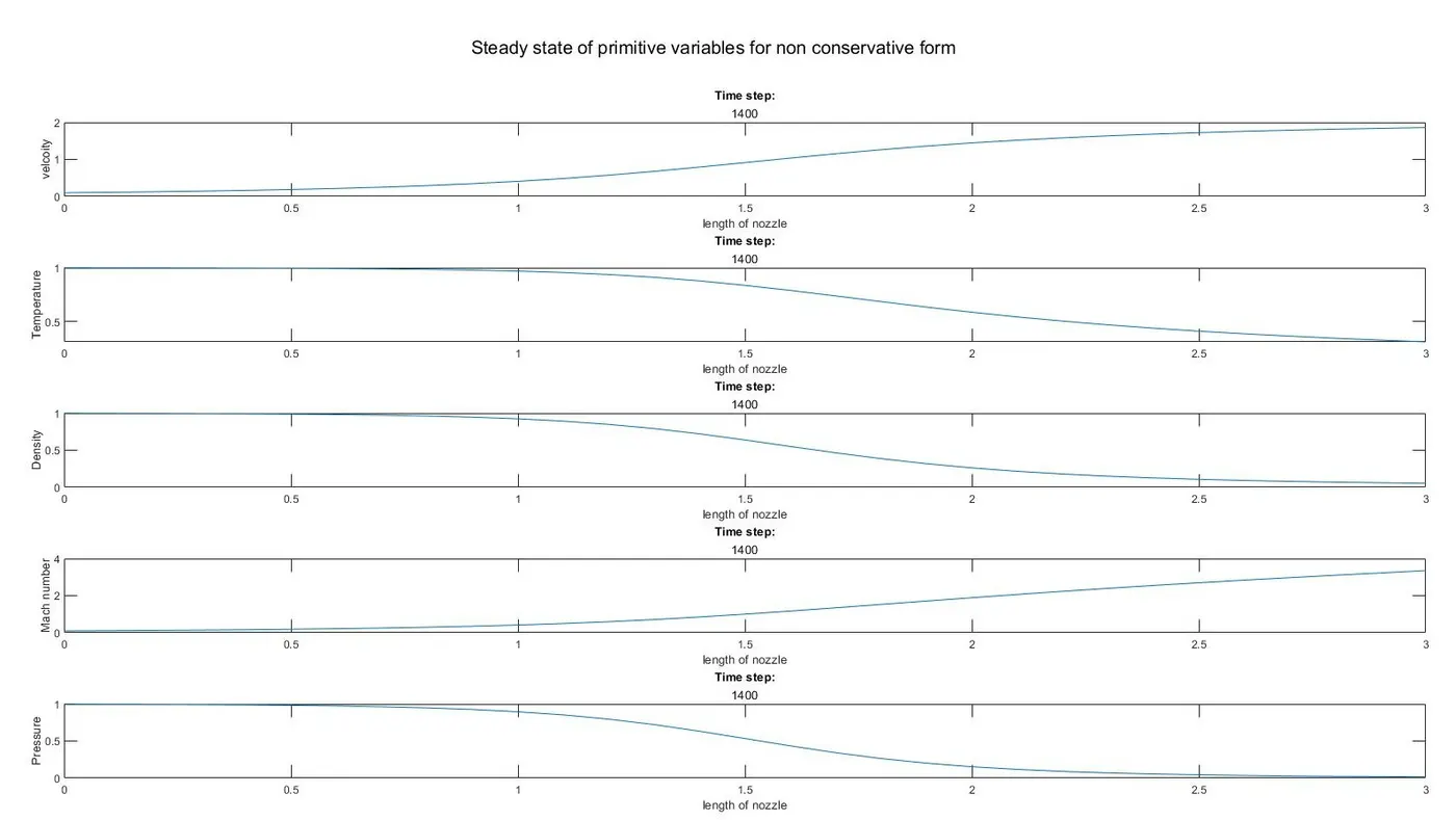
Steady-state distribution of primitive variables with respect to the length of the nozzle.
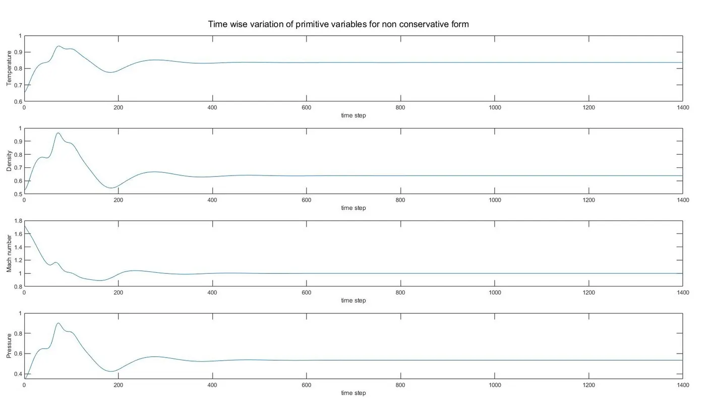
Time-wise distribution of flow variables at different time steps
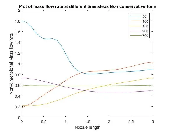
Mass Flow rate at different time steps
Conservation Form
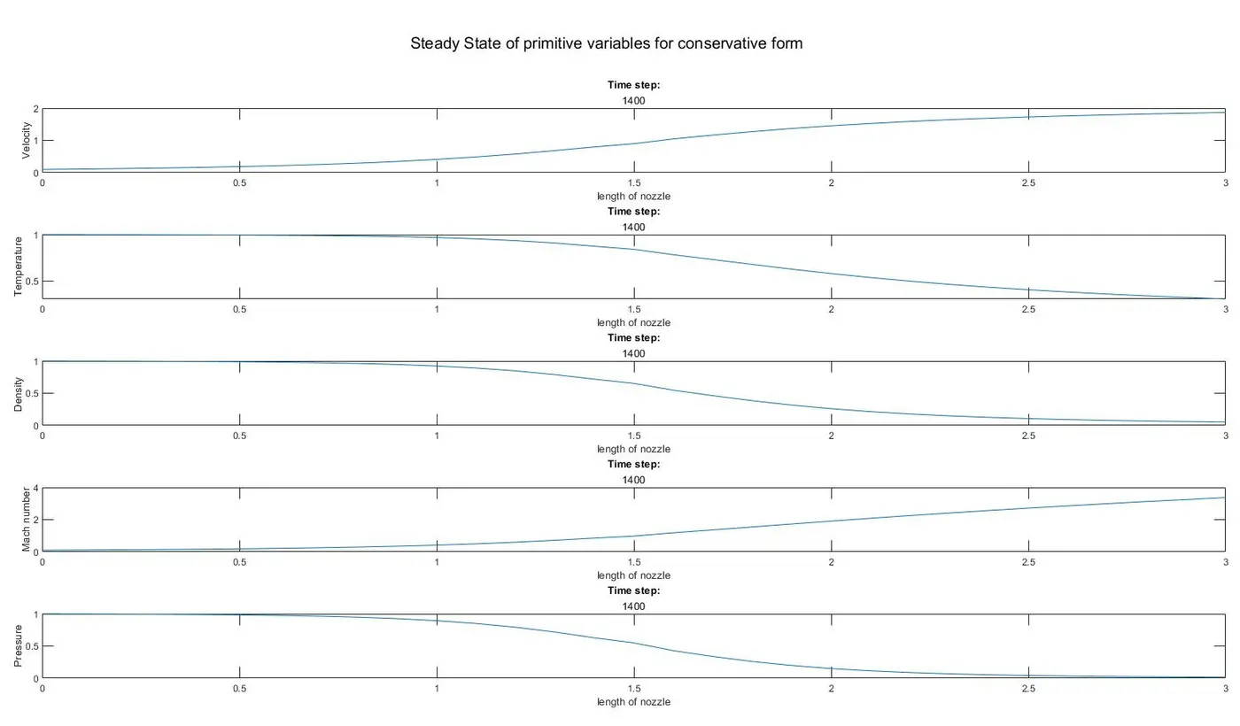
Steady State distribution of flow variables along the nozzle length
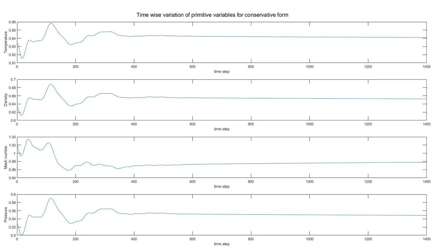
Time-wise variation of flow variables at different time steps
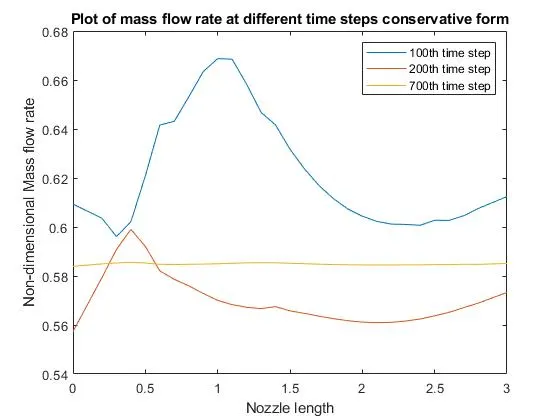
Mass flow rate at different time steps:
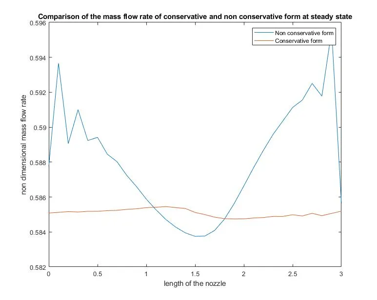
Mass flow comparison of Conservation and non Conservation form at 1400 time steps
Explanation of the Output graph:
The flow variables density, temperature, and pressure decrease along the length of the nozzle whereas velocity and Mach number increases along the length of the nozzle, this type of behavior of the flow are because in the converging part of the nozzle the Mach number is less than 1 as it approaches throat, the area of the nozzle decreases and at the throat, the Mach number is equal to 1. The flow expands isentropically, as a result, the flow accelerates in the divergent part of the nozzle also due to an increase in area and decrease in pressure which results in a decrease in density. Variations in flow variables are high at the initial time steps because the time derivatives are large and oscillate. The oscillations are due to unsteady compression and expansion of waves which propagate through the nozzle. As the time steps increase the flow reaches a steady-state the time derivatives become small and change in the order of six in their magnitude at larger time steps. As the flow attains the steady-state the time derivative becomes zero but when numerically solved this is not achieved. These non zero values are called residuals which are used by CFD experts in comparing the time marching solution of the steady-state with their magnitude and the rate of decay. The same effect can be used to explain the non-dimensional mass flow rate at initial times there are large oscillations of mass flow rate along the length of the nozzle as the flow approaches steady state the mass flow rate is constant which can be seen at a 700th-time step it approaches the steady-state value 0.58 which is close to analytical value.
In the comparison of the mass flow rate between conservation and non-conservation form plot, we can infer that the mass flow rate is closer to the analytical solution. With this, we can say that the conservation form of the governing equations performs well in conserving the mass flow rate than the non-conservation form this is because in the conservation form the mass flow rate is one of the dependent variables whereas in the non-conservation form mass flow rate is calculated from the dependent variables i.e., flow variables.
Conclusion:
1. In conservation form mass flow rate is more conserved which yields a better mass flow distribution whereas non-conservation form results in better-converged solution closer to the analytical solutions this is because of greater decay of the residuals.
2. Non-Conservation form results in accurate flow variables whereas the Conservation form results in accurate flux variables.
3. Computational effort needed for conservation form is more as the flow variables need to be calculated from the solution variables whereas in the non-conservation form the converged flow variables are calculated directly.
4. Conservation form of governing equations is used in shock capturing whereas non-conservation form cannot be applied.
Shock is a sudden change in the flow variables in the direction of flow. The conservation form of governing equations is more suitable in fluid flows that have shocks involved because the primary dependent variables in the equation are the solution variables which results in smooth and stable results whereas in non-conservation form the primary dependent variables are flow variables which result in discontinuous solution during shocks. Hence Conservation form is better than the non-conservation form which involves shock-capturing.
From the above discussion, we cannot conclude the conservative form of governing equations is superior to the non-conservative form or vise versa. The type of governing equations is chosen based on the problem at hand.