Gate Valve Parametric Study

Problem Statement:

1. Perform a parametric study on the gate valve by setting the opening from 10% - 80%.

2. Obtain the mass flow rate and calculate the flow factor and flow co-efficient and plot the same.

3. Discuss the results obtained from the simulation.

Introduction:

Parametric Analysis

It is the study of the influence of different physical or geometry parameters or both on the solution of the model.

Parametric studies allow you to nominate parameters for evaluation, define the parameter range, specify the design constraints, and analyze the results of each parameter variation.

A parametric study requires the following:

• Design Objective is set to Parametric Dimensions
• Parameters nominated for use in the simulation
• Parameter ranges identified
• Design criteria specified
• Various configurations generated

Gate Valve:

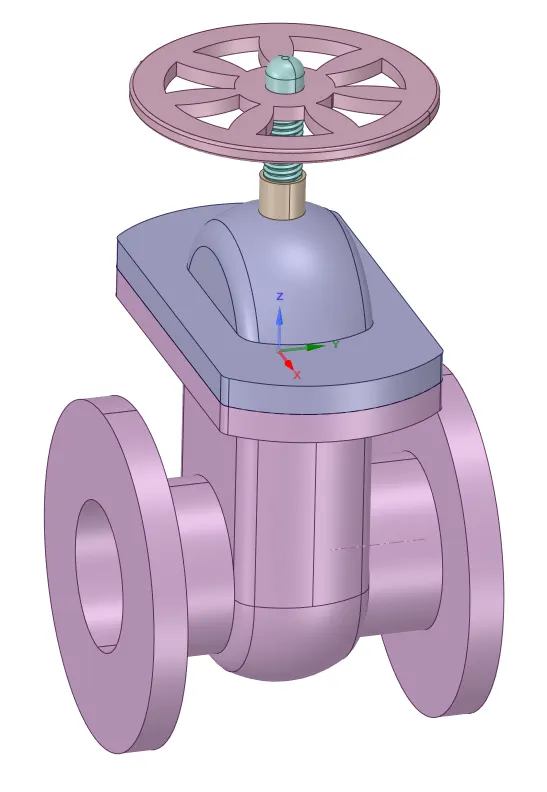
Gate valves are machine elements that are commonly used to control the flow of fluids as the gate valve provides a positive sealing at high pressure of liquids and gases. Gate valves are used when a straight-line flow of fluid and minimum restriction is desired. Gate valves are so named because the part that either stops or allows the flow of fluid through the valve acts as the opening or closing of a gate and is called the gate valve.

Flow Co-efficient

It is a relative measure of the efficiency of the valve in allowing the fluid to flow through it. It is expressed as

`C_v = Q sqrt((SP)/(triangleP))`

where

`C_v` is the flow coefficient measured in PSI drop per gallons per minute

Q - flow rate in gallons per minute

SP - Specific gravity

`(triangleP)` - change in pressure from inlet and outlet in PSI

Flow factor

`K_v = 0.865*C_v` where flow factor is in metric units (`m^3"hr"^-1"bar"^0.5`)

Geometry:

Modified Model:

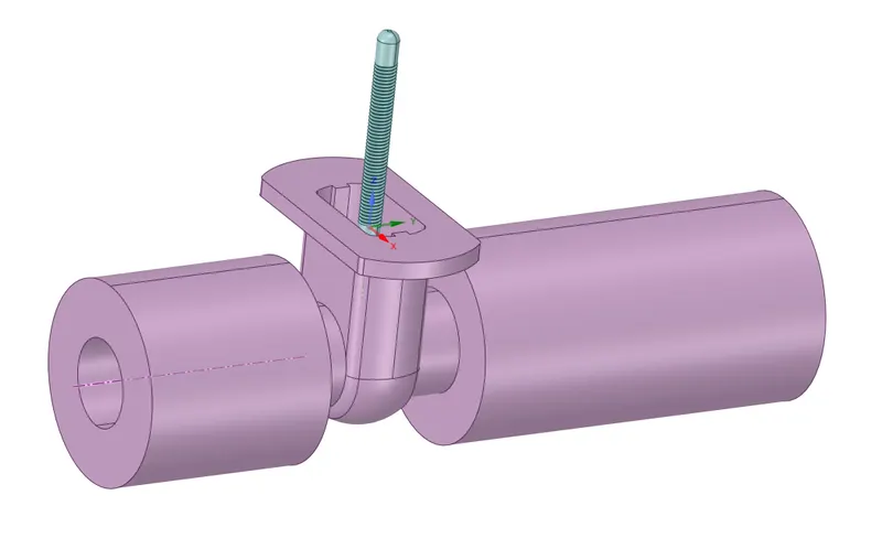
The model is modified such that the short length is the inlet as there is no change in variables involved in the fluid flow and the outlet is extended larger than the inlet as the flow is disturbed by the gate disc and attains a steady-state after a certain length.

Volume Extracted:

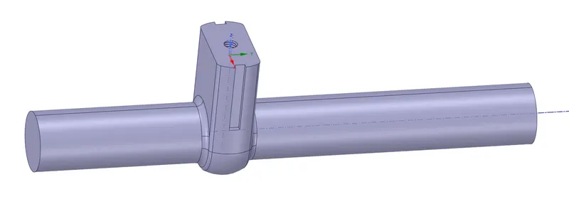
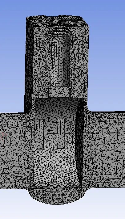
Sectional View of the volume extracted at the elevated gate disc:

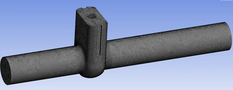
Sectional View of the mesh at the elevated gate disc:

Setting up Physics:

1. Pressure inlet boundary condition is used as the flow rate across the valve is unknown and pressure conditions for the flow are known. At inlet pressure is 10 Pa and outlet 0 Pa.

Pressure Inlet and Pressure outlet boundary condition:

This type of boundary condition is used only when the pressure condition at the inlet is known and other variables such as flow rate are unknown. The inlet pressure used is treated as a loss-free transition from the stagnation condition to the inlet condition. The pressure inputted is the gauge pressure from which the static pressure and the turbulent properties are calculated such as velocity, mass flow rate, etc.,

Pressure outlet boundary condition defines outflow conditions based on the flow pressure at the outlet. This is used when there is a flow rate or higher pressure assigned at the inlet.

2. Realizable K-epsilon turbulence model with scalable wall function is used. Scalable wall function is used to force the log law function in conjunction with the wall function.

3. Water is chosen as the working fluid.

4. Standard initialization is performed with compute from the inlet.

Results:

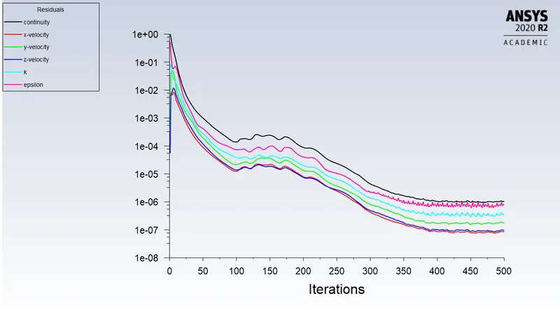
Residual plot:

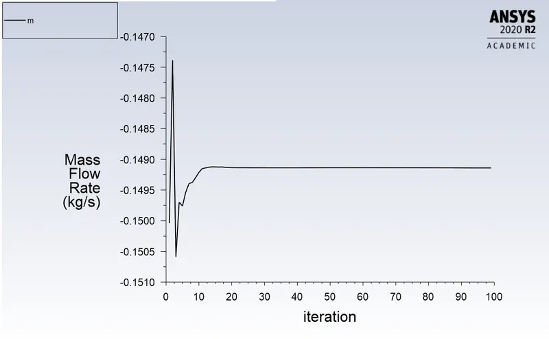
Area weighted average of Mass Flow rate at the outlet.

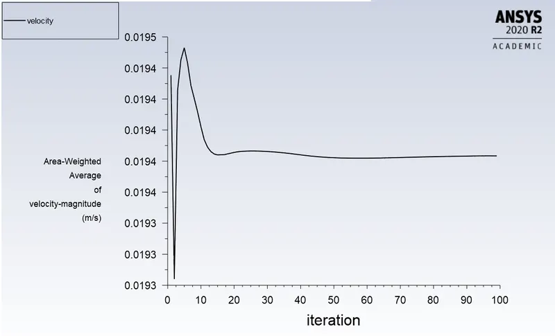
Area weighted average of velocity at the outlet.

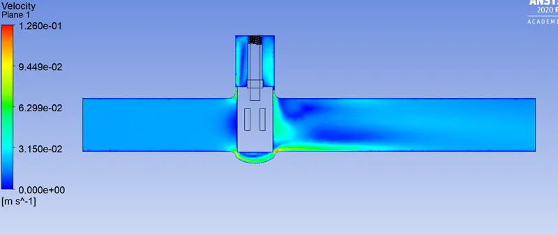
Velocity plot:

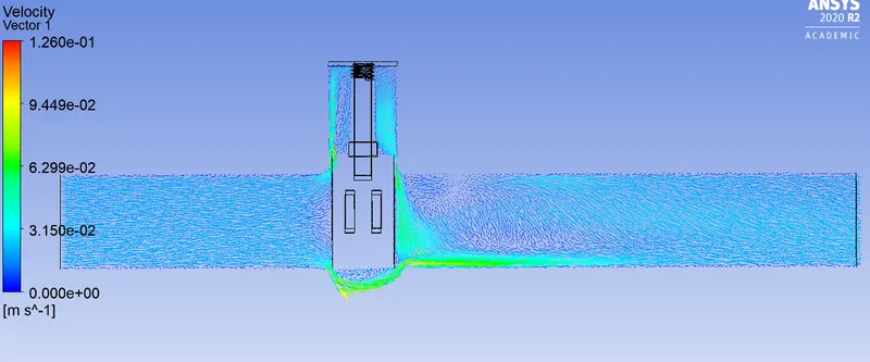
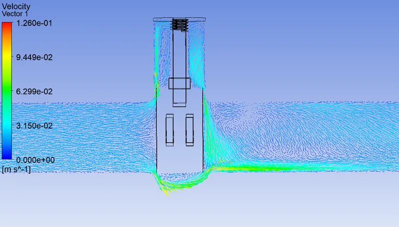
Vector plot for velocity:

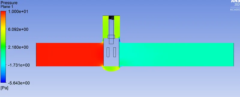
Pressure plot:

Inference:

The pressure inlet condition is defined based on the required flow rate and fluid i.e., water flows from higher pressure to lower pressure is at the outlet. The velocity of the flow is constant from the inlet till the gate disc and increases at the gate disc opening which can be observed from the velocity contour plot and at the exit of the gate disc velocity decrease as there is an increase in the area of the flow due to this there are recirculation regions created near the gate disc. At the recirculation region, the velocity of the fluid is minimum which indicates that the fluid is stagnant at these regions. As the fluid flows towards the outlet it attains the steady-state as in the inlet.

Parametric study on the gate disc:

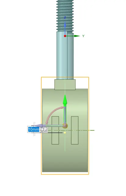
The gate disc is lifted for 10mm from its initial position and assigned as an input parameter which is indicated by the symbol next to the dimension.

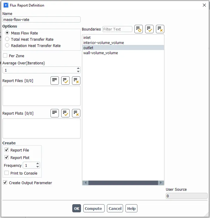
The output parameter is defined when creating the definition for mass flow rate at the outlet in fluent.

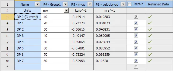
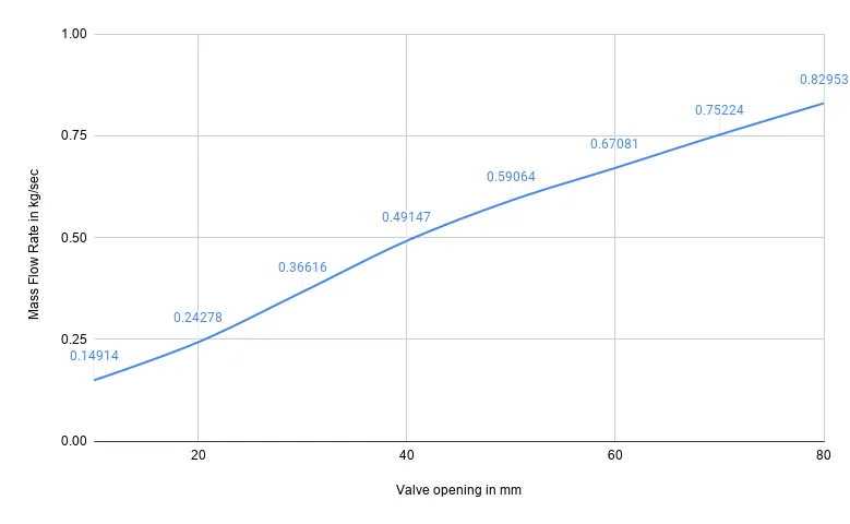
The mass flow rate for different valve opening in mm is calculated using the parametric study.

Calculation of Flow Co-efficient and flow factor for 10% gate valve opening:

Flow Factor `K_v`

`K_v= Q*sqrt((SG)/(triangleP))`

`K_v = 0.14914/998.2*3600*sqrt(1/(1e^-4))`

(Since Q is in kg/sec, it is converted to `m^3`/hr by dividing with the density of water and multiplying 3600 to convert seconds to hours)

`K_v = 53.6904`

Flow Coefficient `C_v`

`C_v = K_v/0.865`

`C_v = 53.6904/0.865`

`C_v = 62.0698`

Similarly, the calculation for flow coefficient and flow factor is performed for different gate valve opening and tabulated in the below table.

Table showing calculated flow coefficient and flow factor for the mass flow rate obtained for different valve opening.

Valve opening in mm	Mass flow rate in kg/sec	Velocity at the outlet in m/s	Flow Coefficient(`C_v`) in GPM/PSI	Flow factor(`K_v`) in `m^3 hr^-1 `bar`^0.5`
10	0.14914	0.019383	62.0698	53.6904
20	0.24278	0.031073	101.041	87.4008
30	0.36616	0.046831	152.390	131.8176
40	0.49147	0.062905	204.542	176.929
50	0.59064	0.075649	245.815	212.6304
60	0.67081	0.085952	279.181	241.4916
70	0.75224	0.096359	313.071	270.8064
80	0.82953	0.10628	345.237	298.6308

The graph plotted between valve opening and flow coefficient and flow factor:

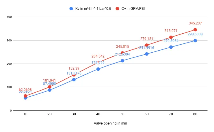
The graph plotted between the Valve opening in mm and the mass flow rate in kg/sec.

Inference:

With an increase in the lift of the gate disc the mass flow rate increases which in turn increases the flow coefficient and flow factor which can be observed from the above plot. It is also observed that the change in the mass flow rate is almost linear with the change in the lift of the gate disc.

Conclusion:

1. At the inlet side of the gate disc pressure is high and decreases as the fluid flows towards the outlet through the gate disc.

2. From the pressure gradient plots we can observe that there is a large pressure change at the gate disc.

3. With increases in the lift of the gate disc the velocity of the fluid at the outlet increases.

4. With increases in valve opening % there is an increase in the mass flow rate, flow coefficient and flow factor.

5. Higher flow co-efficient indicates that the gate valve is more efficient in allowing the fluid to pass through.