Week 5 - Curve fitting

Objective: To create a python script to perform curve fit using the different polynomial models and also apply other methods to fit the curve perfectly with the actual data curve.

Introduction:

Curve fitting examines the relationship between one or more predictors (independent variables) and a response variable (dependent variable), with the goal of defining a "best fit" model of the relationship.

In order to measure the fitness of the curve, the R square method.

In this method SSR = sum of the square of the regression which is the measure of the distance between the data points of the predicted curve and the means of the data points.

Similarly, SSE is a measure of the distance between the original data point and the data point of the predicted curve.

`R^2 = ("SSR")/("SST")`

in order words `R^2 = "explained variation"/"total variation"`

R_square value always lies between 0 to 1.

0 indicates that the model explains no variability of the response data around its mean.

1 indicates that the model explains all the variability of the response data around its mean.

When `R^2`is calculated for the splitwise method polynomial model the value is found to be 0.9999 which explains that the model can explain about 99% of the variation of data about the mean.

1. There are two methods to make a curve fit perfectly

a. Using interpolation

In this method, the curve is drawn through the predicted points one by one. The main drawback is that when the data is generally the points obtained from the data are in place randomly and joining these points one by one will result not result in the meaning full curve. This is method is best suited when the data obtained is reliable.

b. Using error estimation.

Error is the measure of the deviation of the predicted data with the original data. Hence the line with the minimum error is found. One way of finding this line is by increasing the polynomial order to reduce the variations that way the error can be reduced.

Another way is Centering and Scaling.

Standardizing scales the data around 0 with the help of mean and standard deviation. This helps to reduce the multicollinearity of the independent variables which may lead to imprecise coefficients and makes it difficult for the selection of the model.

Normalizing is similar to standardization except instead of dividing them with standard deviation, we only subtract with the mean.

Both normalizing and standardization help reduce the multicollinearity of the independent variables which in turn reduces the error.

In the given problem there is only one independent variable that is Temperature, normalizing, and standardization is unnecessary.

2. The best fit can be done two ways

Splitwise method.

In this method, the entire data points are split into a finite number of sets with each set containing an equal no. of data values. As in this case the total data points are 3200, we split into 5 sets. The coefficients are found separately for each set and the Cp values are predicted for that set. This step is done for all 5 sets individually. Plotting is done between the temperature and Cp values obtained from each set. Since we are limiting the data points to find the coefficients for the model and then predicting Cp values minimum error is generated between the predicted and original values.

Hence splitting the data points to more no. of sets will lead to higher `R^2` values which are the best fit.

Standardization and Normalization

This method is done to reduce the multicollinearity which occurs when independent variables in a regression model are correlated. If the degree of correlation between variables is high it can cause problems during fitting a curve and interpreting the results. The main objective of regression analysis to isolate the relationship between each independent variable and the dependent variable. The regression coefficient represents the mean change independent variable for 1 unit change in the independent variable holding all other independent variables constant.

Increase the degree of the polynomial model.

Problems of Multicollinearity.

If this relationship is not isolated the regression model coefficients values change based on the other independent variables in the model. In other words, the coefficients become sensitive to small changes.

3. Cubic fit can be improved by

1. Splitwise method.

The first step is to identify the points where the square curve intersects the data curve. This intersection indicates that at those points the predicted curve is exactly matching with the raw data curve.

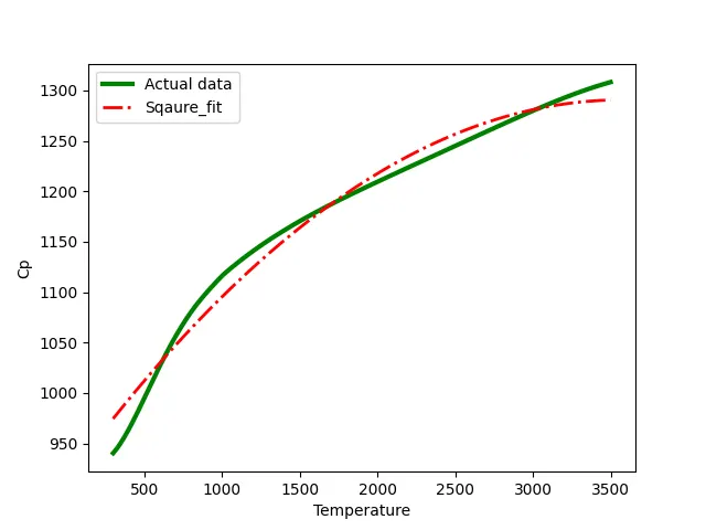
With respect to the above graph, the intersection points are marked. The data points are split with respect to the intersection points. As in this case the data points are split into 5 sets. Coefficients are calculated for each set and Cp values are predicted. The same way coefficients and predicted Cp values for the other 4 sets have been calculated. This is done to reduce the deviation of the predicted curve with the raw data curve.

Standardization.

Standardization is subtracting the mean of the variable from each data points so that mean of the new variable is zero. In this method, the mean of the set of variables is taken for example with respect to the above graph mean of the variables are taken for variables till the first intersection point and standardization is performed on it so that the variation of the predicted curve is less from the raw data curve. This step is performed for all the sets of variables.

1. popt - is a one-dimensional array consisting of optimum values of the coefficients for the polynomial model chosen, each entry matches the order in the function definition.

2. pcov - is the covariance matrix showing the uncertainty and interdependence of each parameter in popt. The pcov variable contains the covariance matrix, which indicates the uncertainties and correlations between parameters. This is most useful when the data has uncertainties

3. np.array(temperature): It generates an array and stores the different values of the temperature and passes the generated value to the numpy for numerical calculation in python.

* in *popt mean: It refers to the value in the array popt

Code which compares the curve fit using the polynomial function of order 2,3,4

#Import the required modules
import math
import matplotlib.pyplot as plt
from scipy.optimize import curve_fit
import numpy as np

#Function definition for 2nd order polynomial
def sq_func(t,a,b,c):
	return a*pow(t,2)+b*t+c

#Function definition for 3rd order polynomial
def cub_func(t,a,b,c,d):
	return a*pow(t,3)+b*pow(t,2)+c*t+d

#Function definition for 4th order polynomial
def quad_func(t,a,b,c,d,e):
	return a*pow(t,4)+b*pow(t,3)+c*pow(t,2)+d*t+e

#Function to extract temperature and cp values from the given data

def data_file():

	temp = []
	cp = []

	for line in open('data','r'):
		values = line.split(',')
		temp.append(float(values[0]))
		cp.append(float(values[1]))

	return temp,cp

#Temperature and its corresponding cp values
temp,cp = data_file()

#Calculating the optimum coefficient values and co-variance values for the polynomial model
popt1,pcov1 = curve_fit(sq_func,temp,cp)
popt2,pcov2 = curve_fit(cub_func,temp,cp)
popt3,pcov3 = curve_fit(quad_func,temp,cp)

# Calculating the cp for the best fit curve
sq_cp = sq_func(np.array(temp),*popt1)
cubic_cp = cub_func(np.array(temp),*popt2)
quad_cp = quad_func(np.array(temp),*popt3)

#Graph plotted for different polynomial model in comparison to actual data.
plt.plot(temp,cp,color = 'green',linewidth =3)
plt.plot(temp,sq_cp,'-.',color = 'red',linewidth =2)
plt.plot(temp,cubic_cp,'--',color = 'black',linewidth =2)
plt.plot(temp,quad_cp,':',color = 'orange',linewidth =2)
plt.xlabel('Temperature')
plt.ylabel('Cp')
plt.legend(['Actual data','Sqaure_fit','Cubic_fit','Quadratic_fit'])
plt.show()

# Fittness of the curve

def fitness(temp,cp,pre_cp):

	for i in range (0,len(temp)):

		mean = np.mean(cp)
		ssr = np.sum(pow((pre_cp[i]-mean),2))
		sse = np.sum(pow((cp[i]-pre_cp[i]),2))
		sst = ssr+sse
		r_sq = ssr/sst
	return r_sq

print("The curve is best fit if R_square is closer to 1")
# To calculate the fittness of the curve for different polynomial model.
R1 = fitness(temp,cp,sq_cp)
print('R_square value for the curve with 2nd order equation', R1)
R2= fitness(temp,cp,cubic_cp)
print('R_square value for the curve with Cubic equation',R2)
R3 = fitness(temp,cp,quad_cp)
print('R_square value for the curve with Quadratic equation',R3)

Explanation:

1. Required modules are import such as math, matplotlib.pyplot, numpy, scipy module for curve fit

2. The polynomial model is defined using functions.

3. Function is defined in order to temperature and cp values from the given data.

4. Optimum values of the coefficients and cp values are found using curve fit command.

5. Predicted cp values are found with the updated coefficient values of the polynomial model.

6. Graph is plotted between the temperature and update cp values.

7. A function is defined to find whether the curve is best fit or not using `R^2` method.

8. If `R^2` is closer to 1 it is termed as best fit.

Code for best-fit curve using splitwise method

import math
import matplotlib.pyplot as plt
from scipy.optimize import curve_fit
import numpy as np

#Cubic polynomial Function
def cub_func(t,a,b,c,d):
	return a*pow(t,3)+b*pow(t,2)+c*t+d
# Quadrilateral polynomial function
def quad_func(t,a,b,c,d,e):
	return a*pow(t,4)+b*pow(t,3)+c*pow(t,2)+d*t+e

#Function to extract temperature and its cp values from the given data.
def data_file():

	temp = []
	cp = []

	for line in open('data','r'):
		values = line.split(',')
		temp.append(float(values[0]))
		cp.append(float(values[1]))

	return temp,cp

#Store the temperature and cp values from the given data.
temp,cp = data_file()

# To calculate the optimum values of co-efficients for the polynomial function
popt1,pcov1 = curve_fit(quad_func,temp[0:625],cp[0:625])
popt2,pcov2 = curve_fit(quad_func,temp[625:1000],cp[625:1000])
popt3,pcov3 = curve_fit(quad_func,temp[1000:1700],cp[1000:1700])
popt4,pcov4 = curve_fit(quad_func,temp[1700:3030],cp[1700:3030])
popt5,pcov5 = curve_fit(cub_func,temp[3030:3200],cp[3030:3200])

# To calculate the cp for the best fit curve
f_cp1 = quad_func(np.array(temp[0:625]),*popt1)
f_cp2 = quad_func(np.array(temp[625:1000]),*popt2)
f_cp3 = quad_func(np.array(temp[1000:1700]),*popt3)
f_cp4 = quad_func(np.array(temp[1700:3030]),*popt4)
f_cp5 = cub_func(np.array(temp[3030:3200]),*popt5)

# Function to calculate the R_sqaure for the temperature its corresponding cp value.
def r_square(temp,cp,f_cp):

	for k in range(0,(len(temp))):
		Mean = np.mean(cp)
		ssr = np.sum(pow((f_cp[k]-Mean),2))
		sse = np.sum(pow((cp[k]-f_cp[k]),2))
		sst = ssr+sse
		r_s = ssr/sst
	return r_s

# To calculate the r_square for each split of the curve
r1 = r_square(temp[0:625],cp[0:625],f_cp1)
r2 = r_square(temp[625:1000],cp[625:1000],f_cp2)
r3 = r_square(temp[1000:1700],cp[1000:1700],f_cp3)
r4 = r_square(temp[1700:3030],cp[1700:3030],f_cp4)
r5 = r_square(temp[3030:3200],cp[3030:3200],f_cp5)

# To find whether the curve is best fit or not
mean_r = (r1+r2+r3+r4+r5)/5

# Displays if the curve is best fit or not
if 0.9<mean_r<1:
	print("The curve is best fit")
else:
	print("The curve is not a perfect fit")


#Plot to show the splitwise method of curve fit
plt.plot(temp,cp,color='cyan',linewidth=3)
plt.plot(temp[0:625],f_cp1,color = 'green',linewidth =2)
plt.plot(temp[625:1000],f_cp2,'-',color = 'y',linewidth =2)
plt.plot(temp[1000:1700],f_cp3,'-.',color = 'red',linewidth =2)
plt.plot(temp[1700:3030],f_cp4,'--',color = 'black',linewidth =2)
plt.plot(temp[3030:3200],f_cp5,':',color = 'orange',linewidth =2)
plt.xlabel('Temperature')
plt.ylabel('Cp')
plt.legend(['Actual data','Quadratic_fit between temperature 0:625','Quadratic_fit between temperature 625:1000','Quadratic_fit between temperature 1000:1700','Quadratic_fit between temperature 1700:3030','Cubic_fit between temperature 3030:3200'])
plt.show()


	

Explanation:

The logic used in this code is the same as before but the coefficient values for the polynomial model are found for a particular range of temperature so that the error induced in find the coefficient values are minimum.

Output:

Plot comparing actual data plot with the different polynomial model

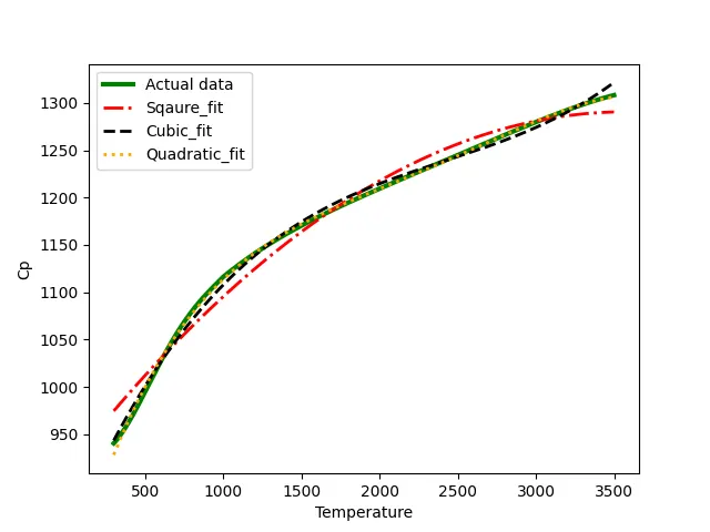
`R^2` values

Plot Showing Splitwise method curve fit

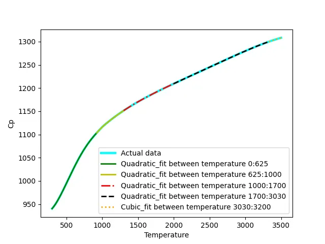
`R^2` value

Conclusion:

From the `R^2` value obtained from the different polynomial models and splitwise method, it can be inferred that `R^2` is closer to 1 which represents the best fit when compared to use of higher degree polynomial models.