Mixing efficiency
Problem Statement: Create a steady-state simulation to compare the mixing effectiveness when hot inlet temperature of 36 degree celius is mixed with the cold inlet at 19 degree celius.
Use a suitable RANS turbulence model for the simulation under different inlet conditions.
Introduction:
T junction is formed when two pipes are jointed perpendicular to each other. It has wide range of applications from house hold plumbing to Air condition ducts in industries etc. As the flow considered is turbulent in this study Reynold average Navior Strokes equation is used. RANS is further divided into several models which can be chosen according to the problems. Among the several models in RANS K-epsilon and K-omega turbulence models are used in this study.
K epsilon is two equation RANS turbulence model, in this model we solve for two variables, turbulent kinetic energy k and turbulent dissipation of kinetic energy epsilon. This model uses wall functions to account for the fluid velocity in the viscous sublayer near the wall.
Main limitations for K-epsilon models are:
- No-slip walls.
- Adverse pressure gradients.
But varies models in K-epsilon models were developed to improve the performance of K-epsilon model. They are Realizable K-epsilon model, RNG K-epsilon model.
K-omega is another turbulence model where rate of dissipation of kinetic energy epsilon is replaced by omega. The main objective of this model is to account for near wall interactions more accurately than K-epsilon model.
Limitations for K-omega
- Difficulty of convergence compared to K-epsilon
- Sensitivity to initial conditions.
Due to these limitations K-omega SST model was developed. This model is an hybrid of K-omega and K-epsilon model. This model is used mainly in aeronautics area where freestream turbulence levels has to be addressed and it can also applied to the viscous affected region without further modification.
Simulations is done for Tee junction under following cases to compare the results of K-epsilon and K-omega turbulence models.
- Case 1 for short length
Hot air inlet velocity 3m/s.
Momentum ratio 2.
- Case 2 for short length
Hot air inlet velocity
Momentum ratio 4.
Formula:
``Momentum ratio = (Velocity of Cold inlet)/ (Velocity of Hot inlet)``
Procedure:
1. To extract volume open space claim, under prepare menu use volume extract command and select the edges of the geometry and suppress the uploaded step file.
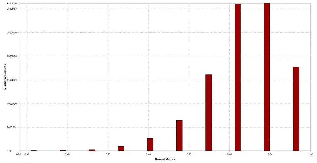
2. Open the mesh window and enter the mesh parameters and generate the mesh and also check for quality of the mesh which should not be less than 5%. Update the mesh window at the end
3. Open the setup window to select the turbulent models and enter the initial and boundary conditions under physis menu.
4. To plot the graph of weighted average temperature and standard deviation we need to define it in definitions under solutions window.
5. Initialze the model under use defined menu to calculate the values for initial time step and then enter the number of iterations to perform.
Geometry
Given step file is opened in SpaceClaim in to extract the volume using extract volume under prepare menu. 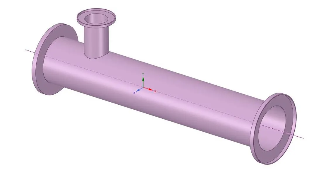
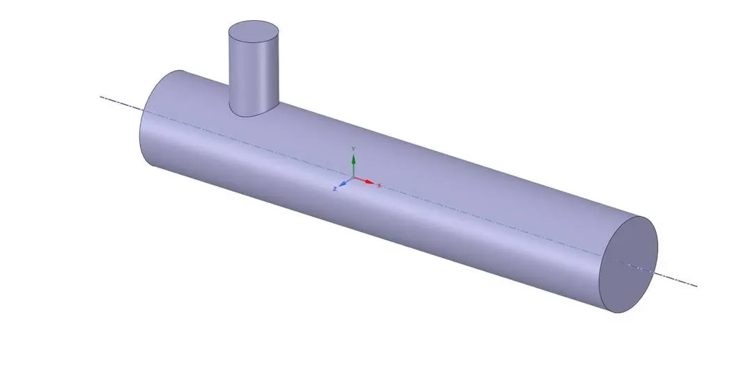
Extracted Volume.
Meshed model with mesh cell size of 2mm.
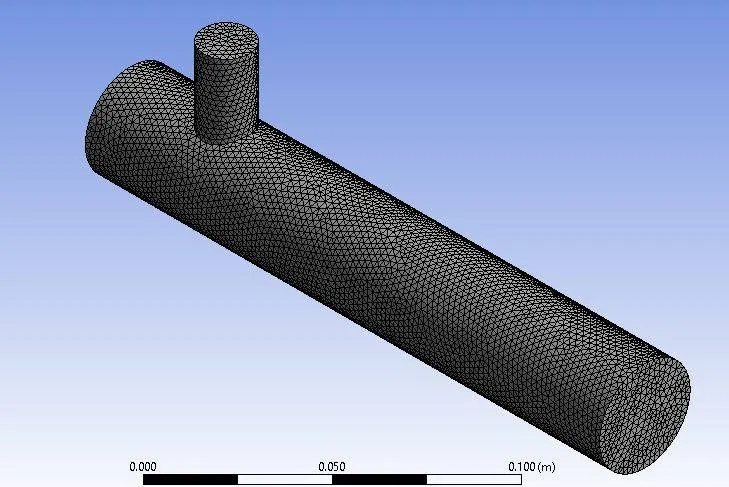
No. of cells = 105836
Nodes = 21342
Mesh quality:
Initial and Boundary conditions
Boundary condition used is Velocity inlet and pressure outlet.
|
Boundary |
Variables |
Values |
Unit |
|
Inlet_x |
Velocity |
3 |
m/s |
|
Temperature |
36 |
celius |
|
|
Inlet_y |
Velocity |
6 |
m/s |
|
Temperature |
19 |
celius |
|
|
Outlet |
Pressure |
0 |
Bar |
|
Wall |
NA |
No slip condition |
NA |
Named selection from mesh window
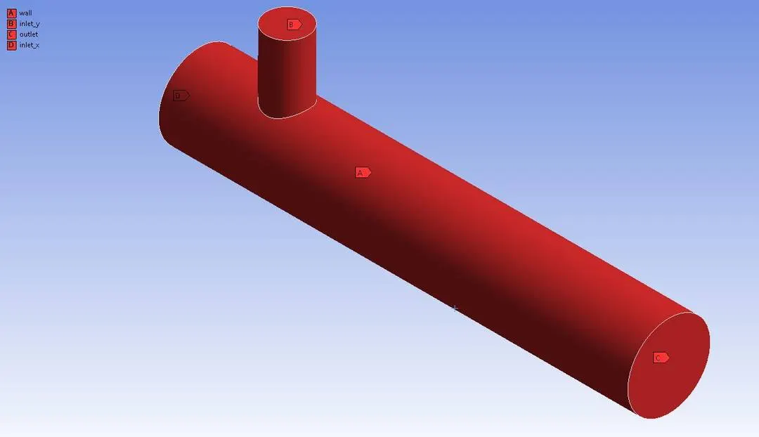
With the above Initial and Boundary conditions simulation is done for K epsilon and K omega
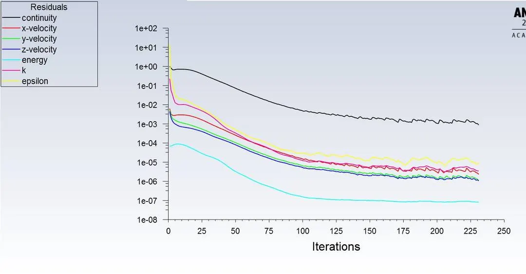
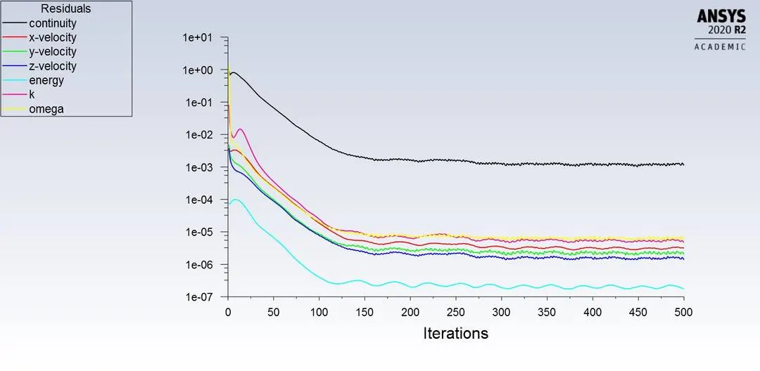
Below are the plots for K-epsilon and K-omega for momentum ratio 2 for short Tee model.
Residuals plots K epsilon
Residual plots for K-omega
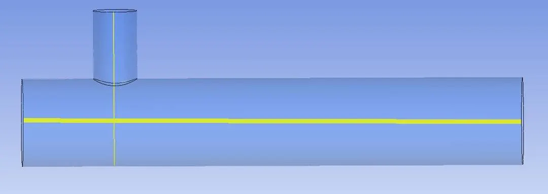
Line probe along length of the pipe and at the T junction.
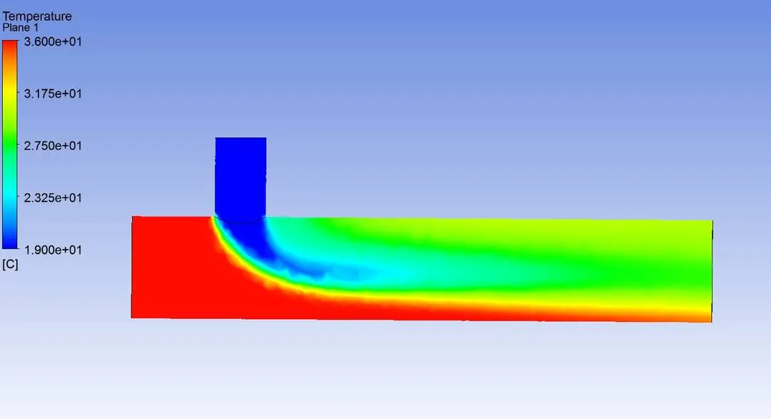
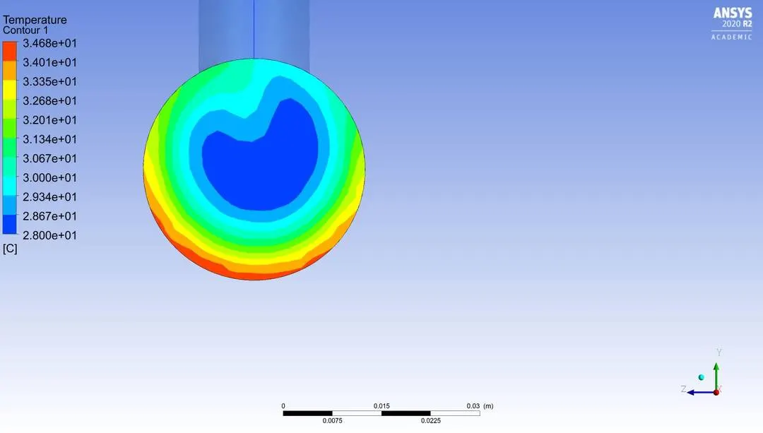
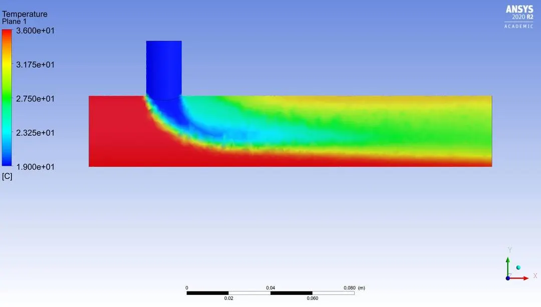
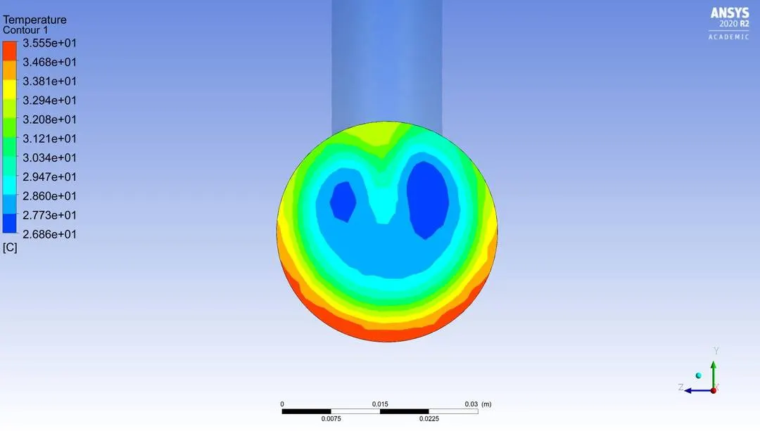
Temperature plot along the length using plane parallel to xy plane
K-epsilon
K-omega
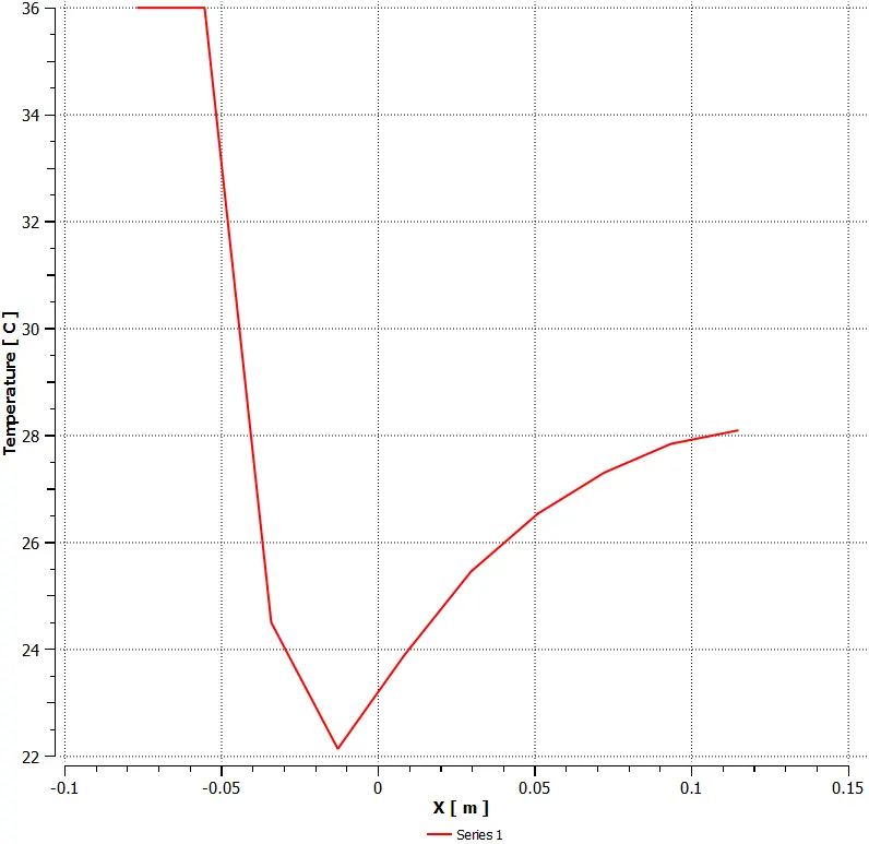
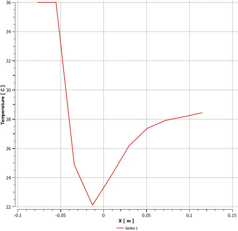
Temperature graph using line probe along the length
K-epsilon
K-omega
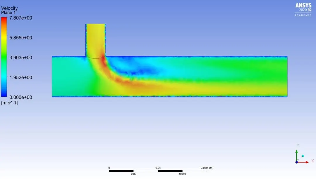
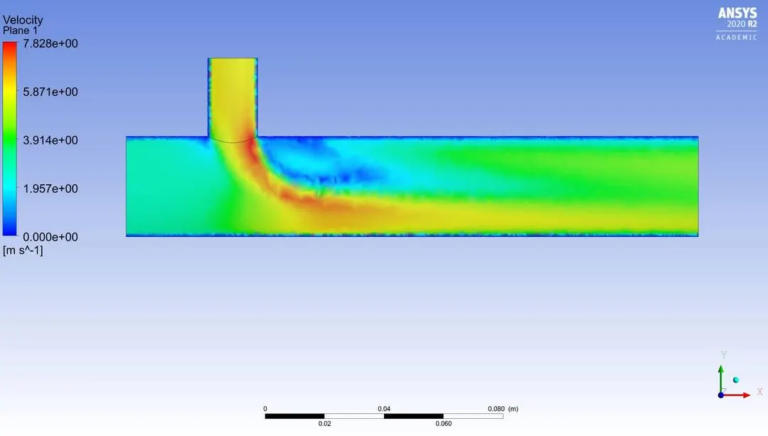
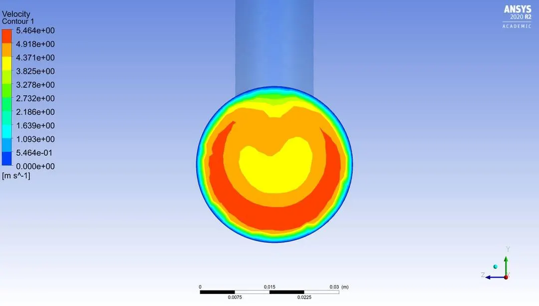
Velocity plot along the length using plane parallel to xy plane.
K-epsilon
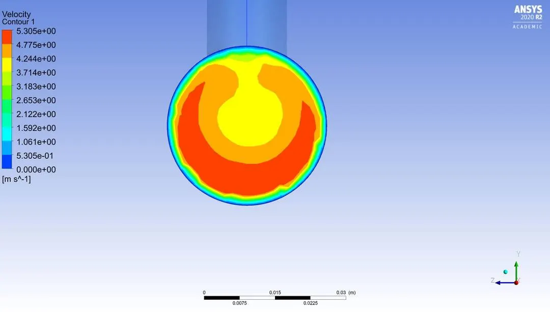
K-omega
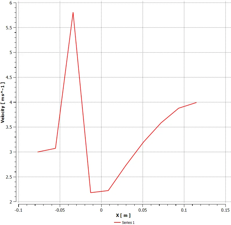
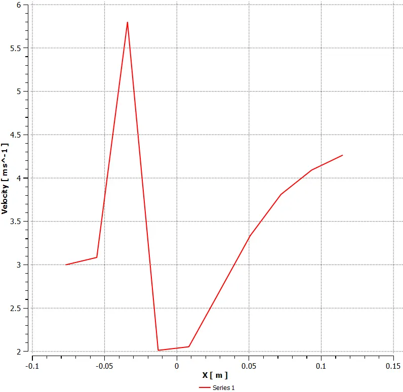
Velocity graph along the length using line probe.
K-epsilon
K-omega
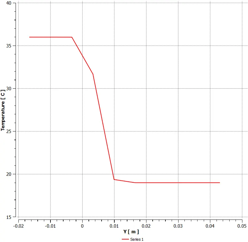
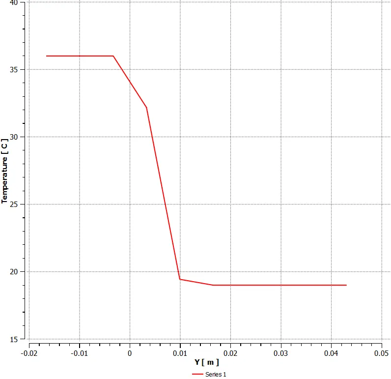
Temperature at T junction
K-epsilon.
K-omega
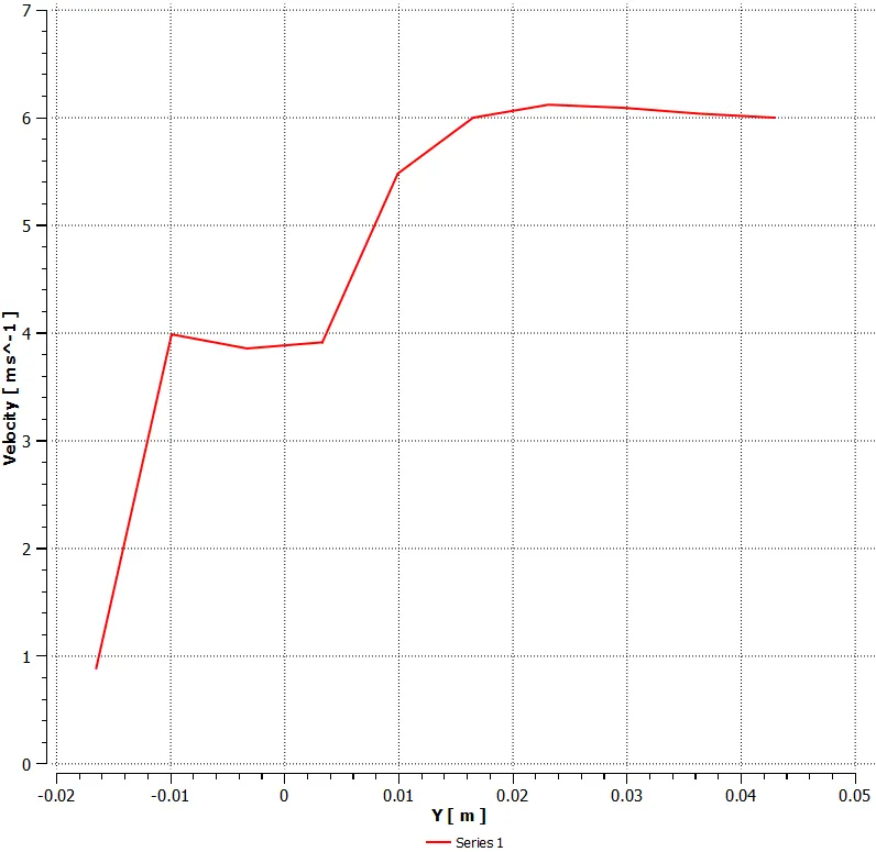
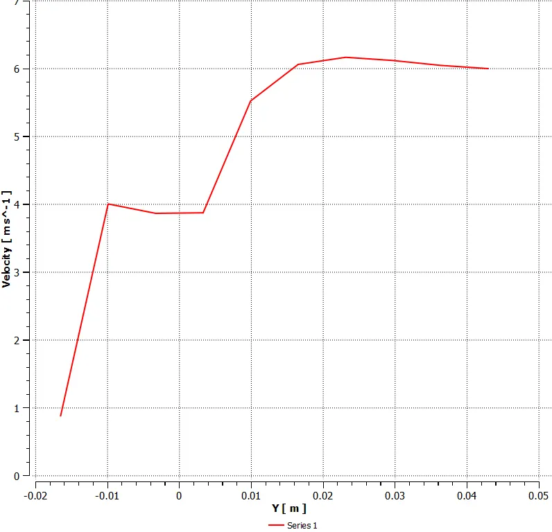
Velocity at T junction
K-epsilon
K-omega
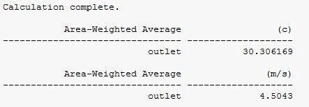
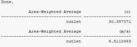
Weighted average values for temperature and velocity printed in console panel.
K-epsilon
K-omega
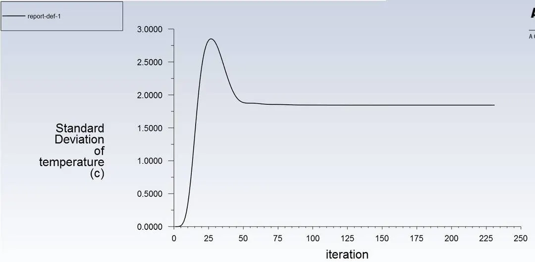
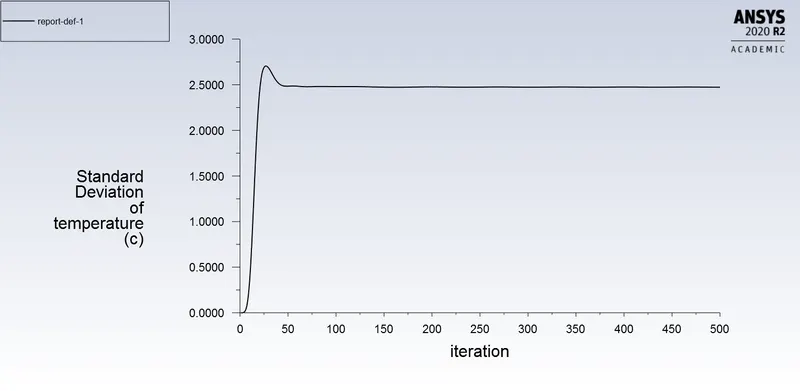
Standard deviation for temperature at outlet
K-epsilon
K-omega
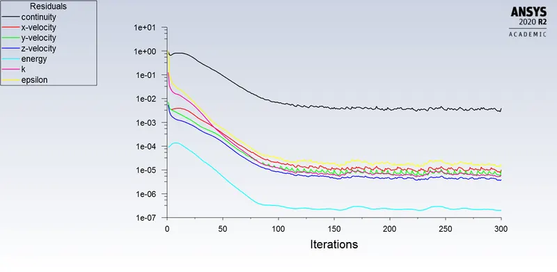
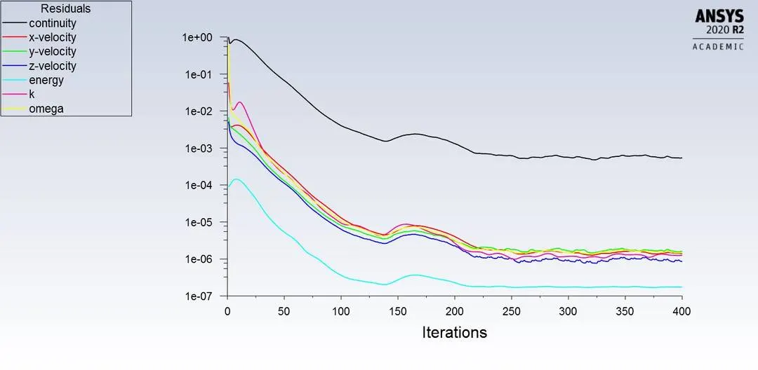
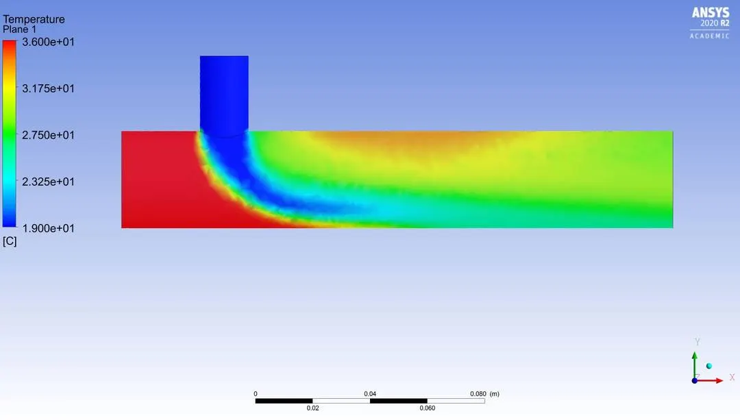
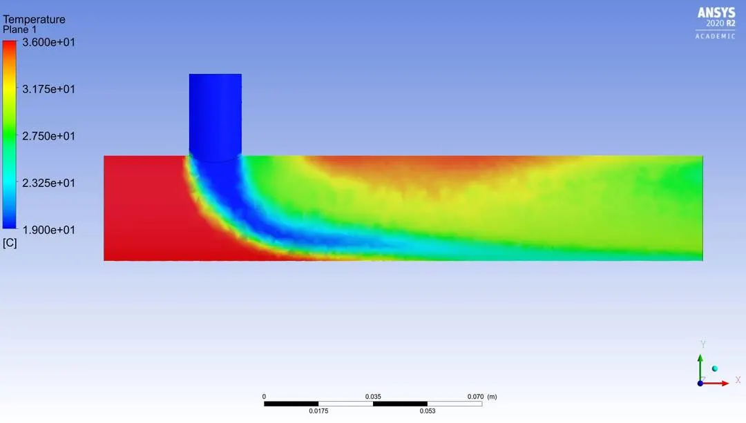
Simulation for momentum ratio 4 for short Tee model.
Residual plots
K-epsilon
K-omega
Temperature plot along the length
K-epsilon
K-omega
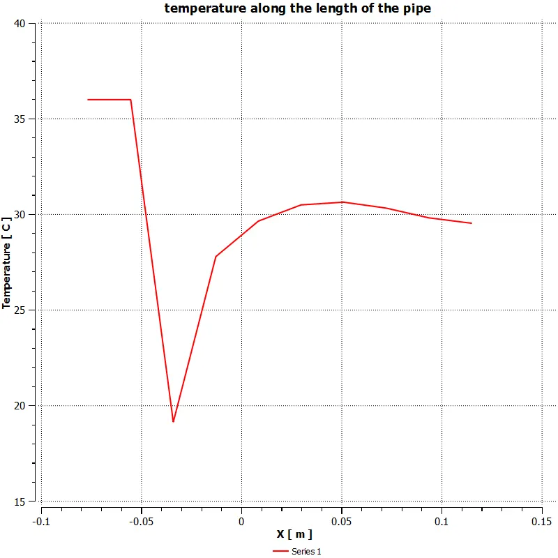
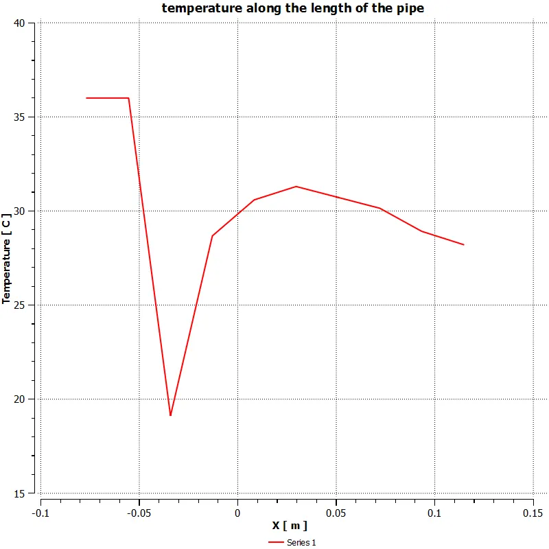
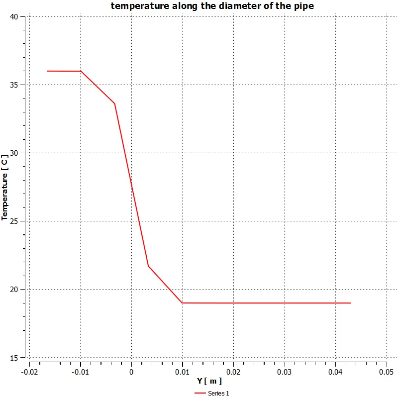
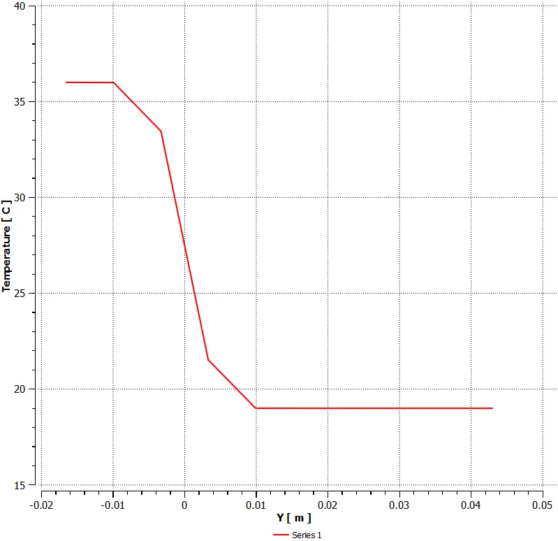
Temperature graph along the length
K-epsilon
K-omega
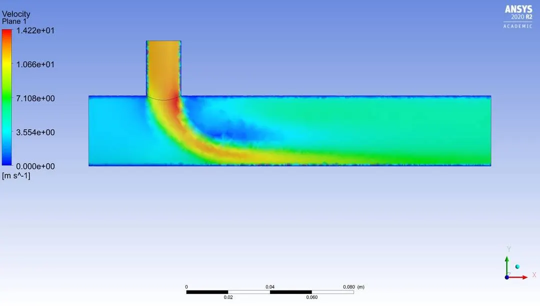
Velocity plot along the length
K-epsilon
K-omega
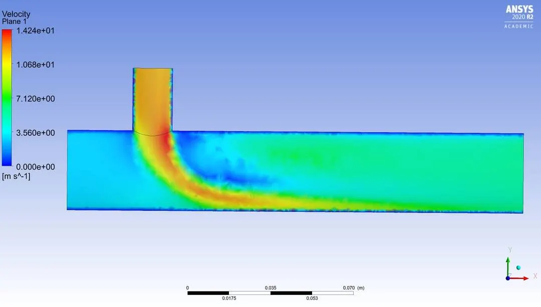
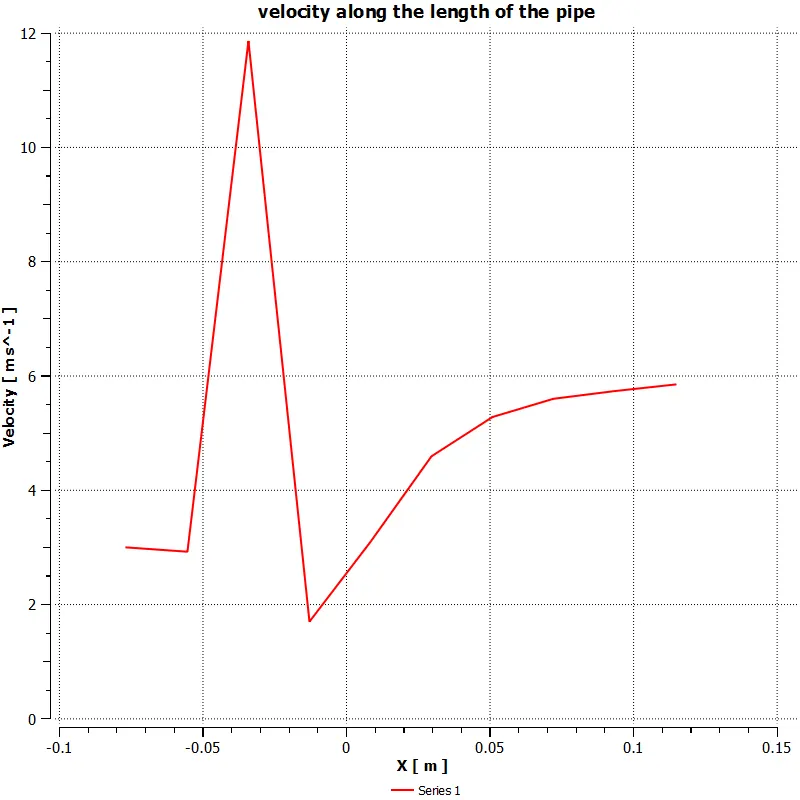
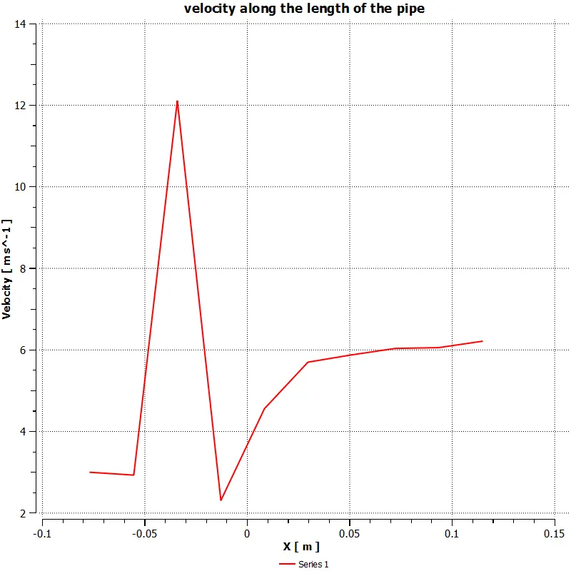
Velocity plot along the length
K-epsilon
K-omega
Temperature at T junction
K-epsilon
K-omega
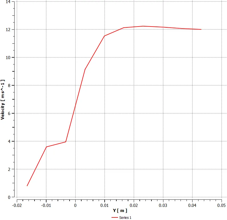
Velocity at T junction
K-epsilon
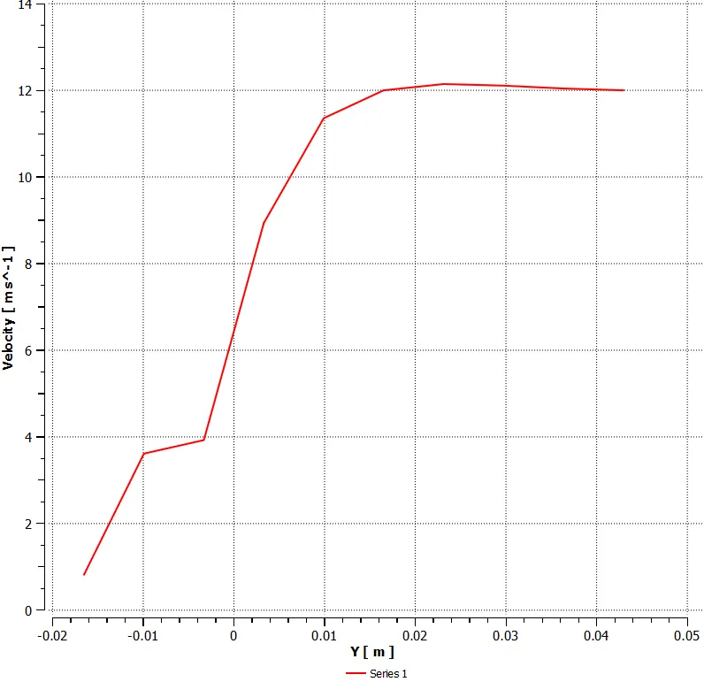
K-omega
Weighted average values for temperature and velocity
K epsilon
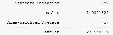
K-omega
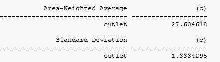
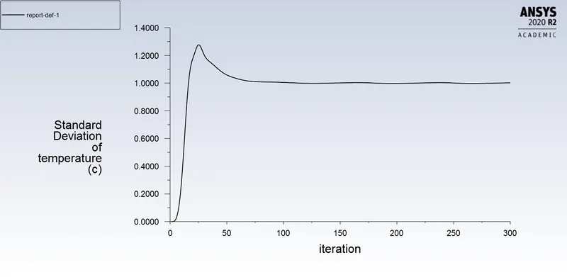
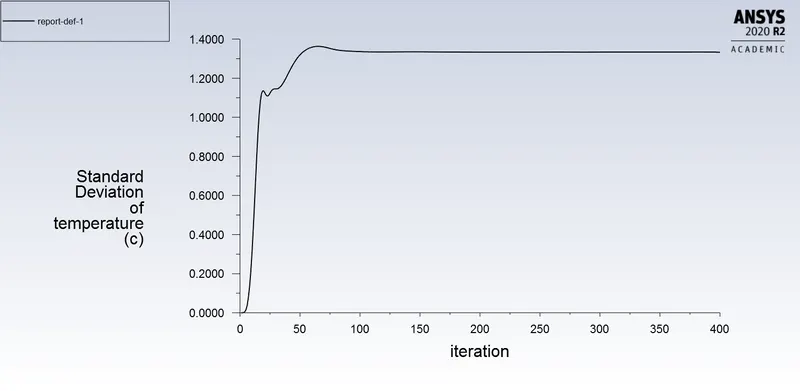
Standard Deviation of the outlet temperature
K-epsilon
K-omega
Inference:
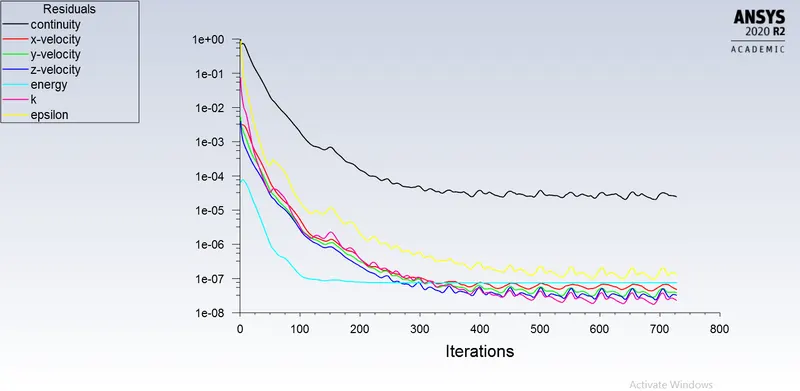
From the above plots we can infer that the converged solution varies in the order of `10^-2` between K-epsilon and K-omega turbulent models and also the mixing efficiency is higher is K-epsilon model which is supported by Standard deviation plot, Higher the Standard deviation lower is the mixing efficiency and vice versa. From the residulas plots K-epsilon takes less no. of iterations when compared to K-omega model and also high Reynolds number is involved in which K epsilon results more accurate solution than K-omega and y+ values are above 5 which favors for K-epsilon turbulence models. Hence for this problem K-epsilon turbulent model is suitable.
For momentum ratio 4, mixing efficiency is more which can be observed from the standard deviation plot (Higher standard deviation means low mixing efficiency and lower standard deviation means higher mixing efficiency) and the results obtained are closer to analytical solution.
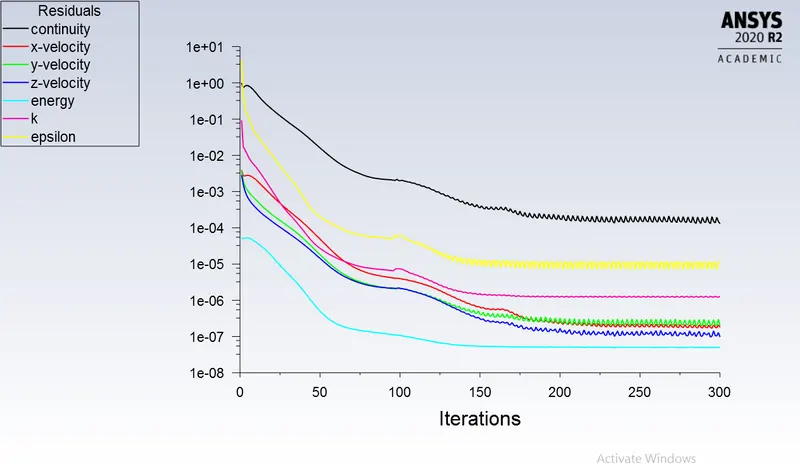
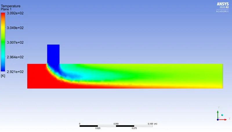
Simulation for long Tee with momentum ratio 2 using K-epsilon turbulent model.
Residual plot
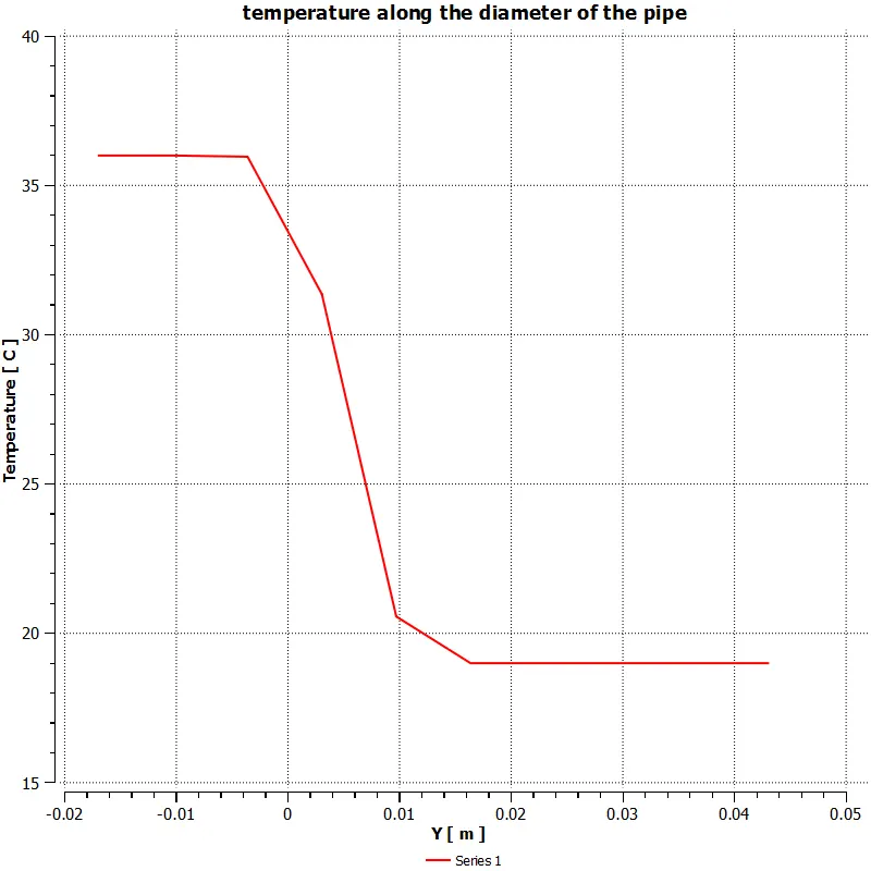
Temperature plot along the length
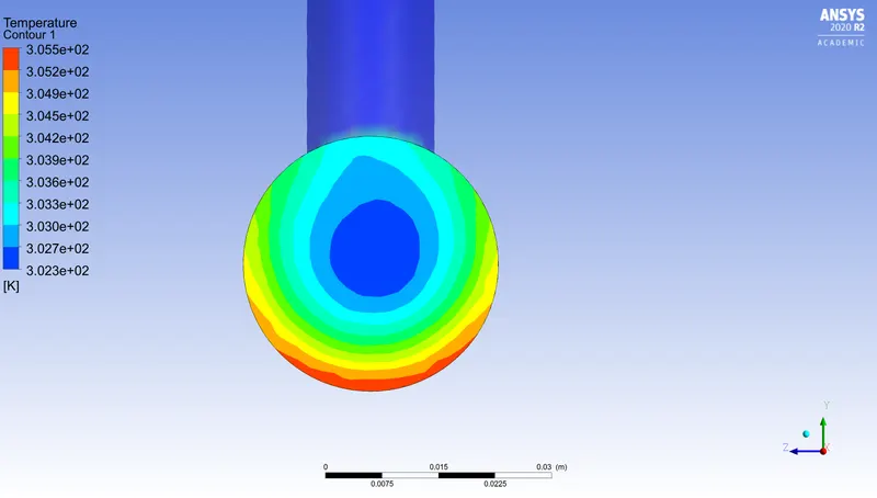
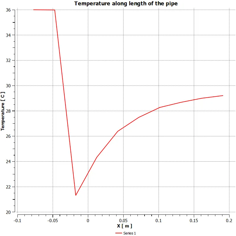
Temperature graph along the length
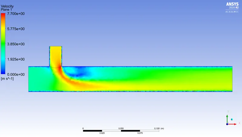
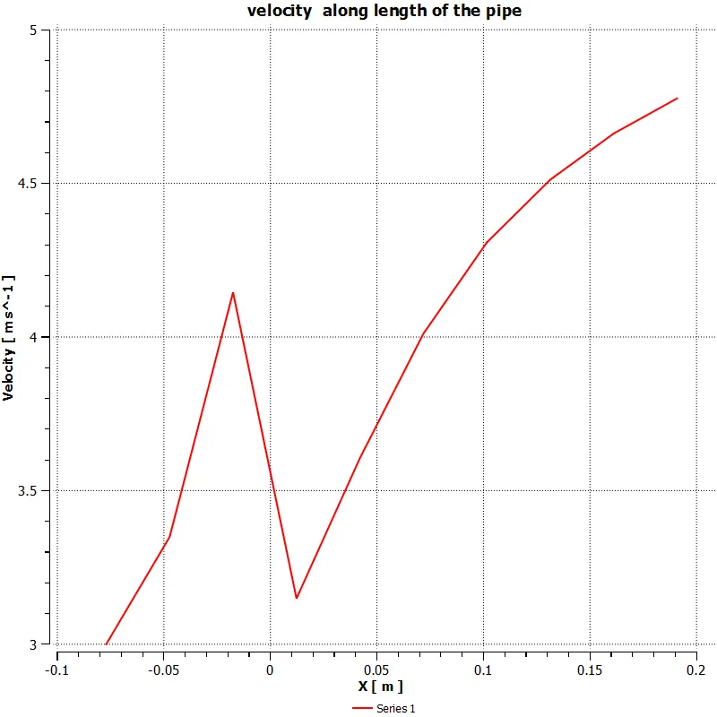
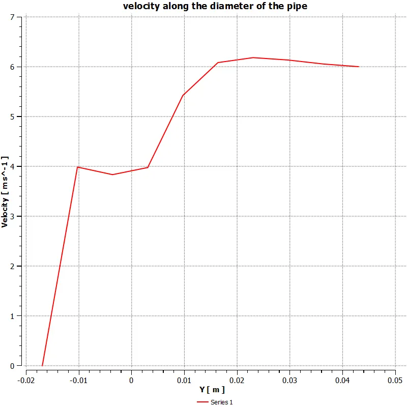
Velocity plot along the length
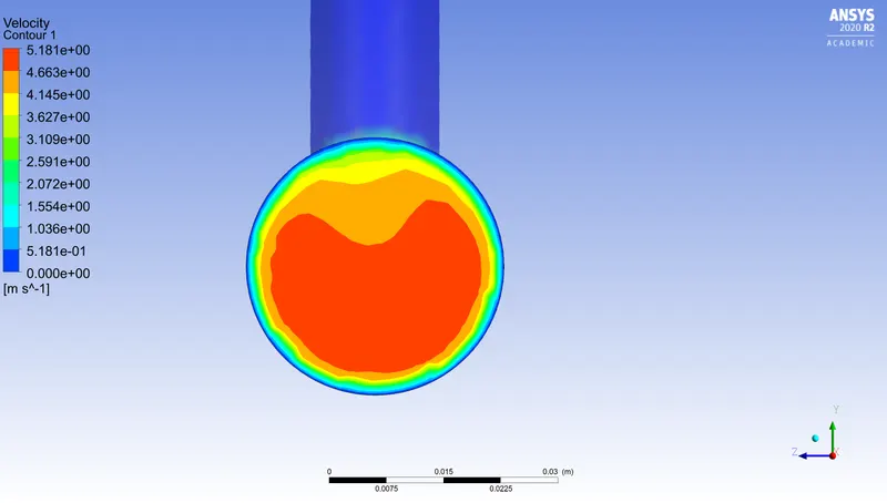
Velocity plot along the length
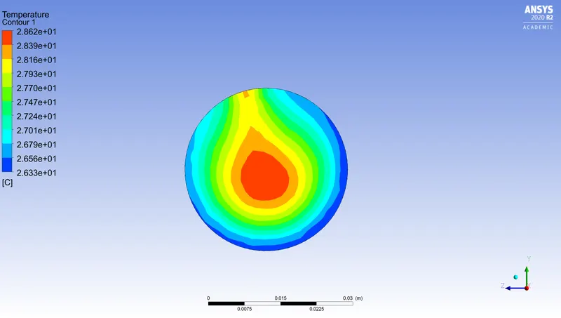
Temperature at the T junction
Velocity at the T junction.
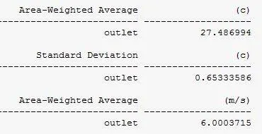
Weighted average values for temperature and velocity
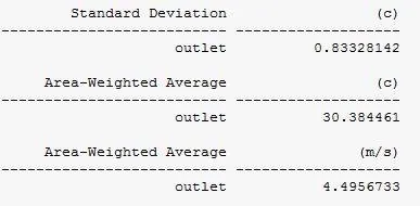
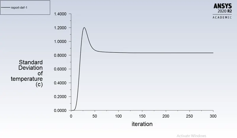
Standard deviation for temperature at outlet
Simulation for long Tee with momentum ratio 4
Residual plot
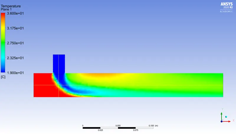
Temperature plot along the length
Temperature graph along the length
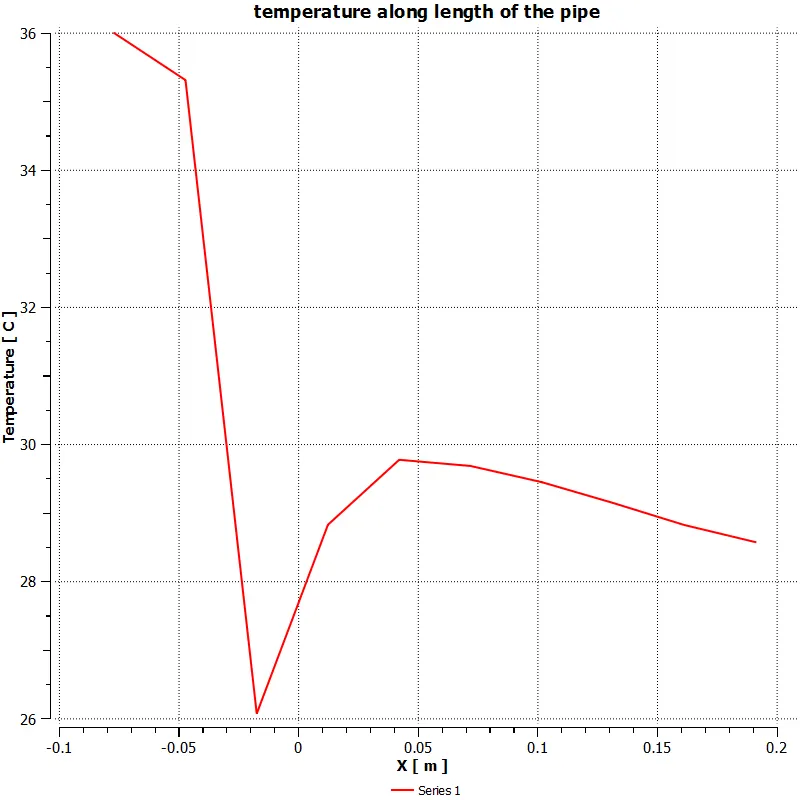
Velocity plot along the length
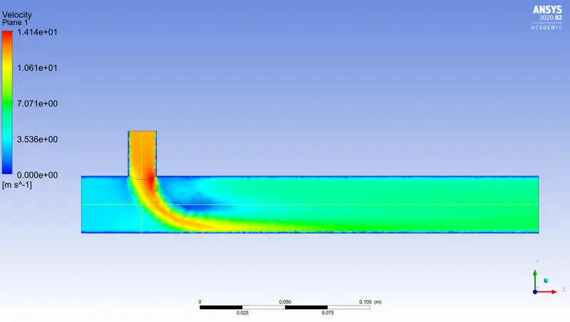
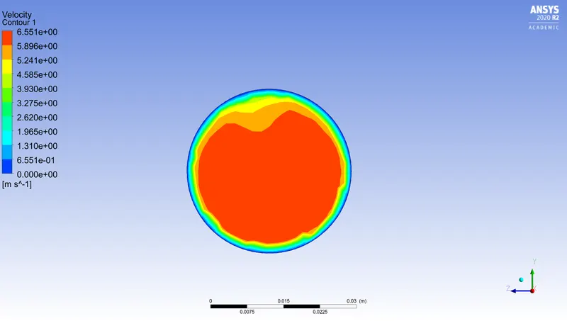
Velocity plot along the length
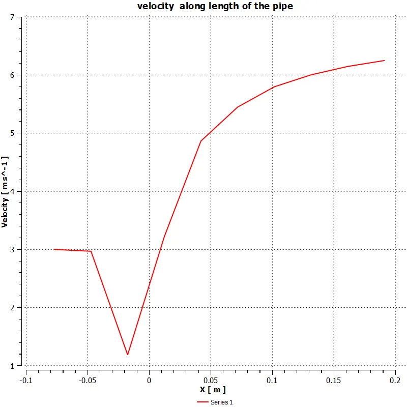
Temperature at T junction
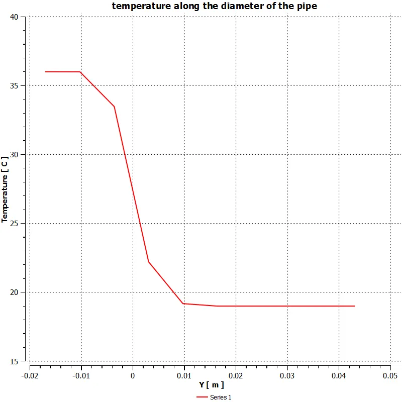
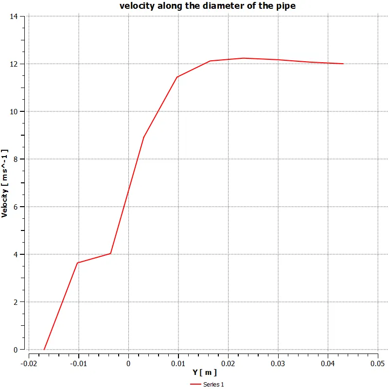
Velocity at T junction
Weighted average values for temperature and velocity
Standard Deviation at the outlet temperature.
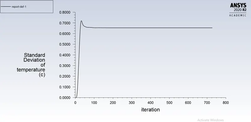
Table Comparing mixing efficiency of short tee and long tee model for K-epsilon turbulence model.
| Model type | Momentum Ratio | Standard Deviation |
| Short Tee | 2 | 2.25 |
| Short Tee | 4 | 1.0002 |
| Long Tee | 2 | 0.8 |
| Long Tee | 4 | 0.6 |
Inference:
From the above plots the variation of temperature and velocity for the given momentum ratio does not vary when compared with the short Tee. However from standard deviation at the outlet temperature decreases indicating higher mixing efficiency with increase in length.
Grid Independence test
In order to verify that the results obtained from the simulation do not vary with size of the mesh, no. of mesh cells are varied by increasing the mesh element size.
|
Type |
Turbulence model |
Mesh cell size |
Cell Count |
Y+ range |
Weighted Average outlet temperature (celius) |
No. of iterations |
|
Short Tee with momentum ratio 2 |
K-epsilon |
1.5mm |
211968 | 4-14 | 30.35 | 280 |
|
2 mm |
105836 | 6-16 | 30.30 | 230 | ||
|
5 mm |
14330 | 10-30 | 30.27 | 200 |
From the above table we can observe the y+ value range increases as the mesh cell size increases because of which K-epsilon turbulent models results more accurate solution which can be seen from the average temperature values at the outlet of the tee model.
Conclusion
1. Comparing mixing efficiency, K-epsilon turbulent mixing efficiency is higher than K-omega turbulent model.
2. K-epsilon turbulent model takes less no. of iterations to converge than K-omega turbulent model.
3. With increase in momentum ratio the outlet temperature approaches closer to analytical solution where inlet velocity of cold air increases.
4. With increases in the length of the model the mixing efficiency increases .