Steady Vs Unsteady flow over a cylinder
Problem Statement:
- Simulate flow over a cylinder for different Reynolds number by varying the velocity of the flow using steady solver and calculate the drag and lift coefficient.
- Simulate the flow over a cylinder for steady and unsteady solver and calculate the Strouhal Number for Re 100.
- Study and discuss the effect of Reynold number on the coefficient of drag.
- explain the effect of Von Karman Vortex street.
Introduction
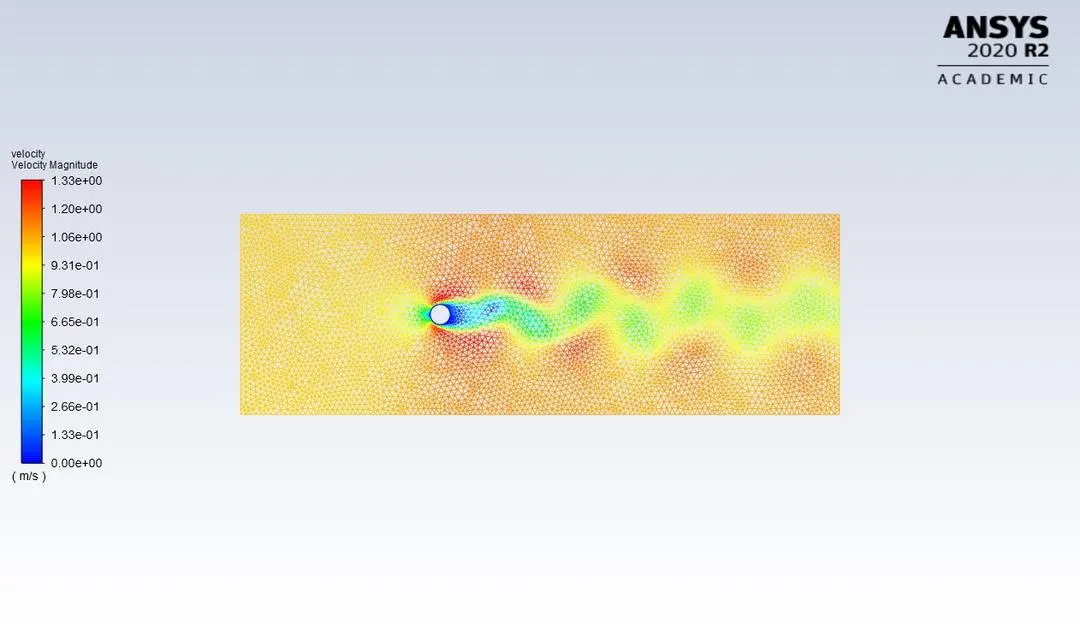
Flow over a blunt body such as circular cylinder experiences boundary layer separation and flow oscillations in the wake region behind the body. When Reynolds number exceeds a threshold value flow motion developed in the wake region behind the body is a result of boundary layer separation from both the sides of the body. This pattern of separation is called Von Karman Vortex Street. A Von Karman vortex street is repeating patterns of swirling vertices that are arising in the wake of flows around the blunt objects. The frequency of these oscillations is related to the Reynolds number of the flow which in this case depends on the velocity of the inlet flow.
Vortex Shedding:
Vortex shedding is an oscillating flow that takes place when a fluid flows past a blunt body at certain velocity. In this flow the boundary layer separated from the surface forms a shear layer which roll into vortex and detach from the surface whereas in Von Karman Vortex Street shedding occurs from both the sides of the body which interact with each other. They shed alternatively from the cylinder and generates a regular vortex pattern called Karman Vortex Street.
Strauhal Number:
Strauhal number is the non dimensional number describing the oscillating flow mechanism.
`Sr = (f*L)/v`
where Sr is Strauhal Number
f - frequency of oscillation in Hz
L - characteristic length in m.
In this case L = D, where D is the diameter of the cylinder in m.
v - velocity in m/s
Large Strauhal number indicates that the viscosity dominates the flow whereas lower Strauhal number indicates high speed fluid.
Drag Coefficient.
Drag Coefficient is a dimensionless quantity that is used to quantify the resistance of an object. It is used in the drag equation which lower drag coefficient indicates less aerodynamic or hydrodynamic drag.
Formula for Coefficient of drag (`C_d`):
`C_d = (2.F_d)/(rho.V^2.A)`
where `F_d` is drag force in N.
`rho` - density of the material in Kg/`m^3`
V - velocity of the inlet flow in m/s
A - area of the object in `m^2`, here A is area of cylinder with diameter 2m.
Lift Coefficient.
Lift coefficient is non dimensionaless quantity that relates to the lifting force to the density of the fluid and velocity of the fluid and associated area of the object.
Formula for Coefficient of lift(`C_l`):-
`C_l = (2.F_l)/(rho.V^2.A)`
Where `F_l` is the lift force in N.
`rho` - density of the material in Kg/`m^3`
V - velocity of the inlet flow in m/s
A - area of the object in `m^2`, here A is area of cylinder with diameter 2m.
Procedure:
Modelling of the Geometry:
Dimensions of the Geometry:
Total length = 60m.
Total Width = 20m
Diameter of the cylinder = 2m.
Distance between inlet and center of the cylinder = 10D = 20m.
Distance between outlet and center of the cylinder = 20D = 40m.
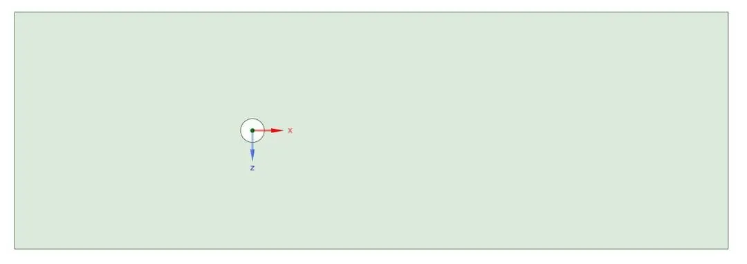
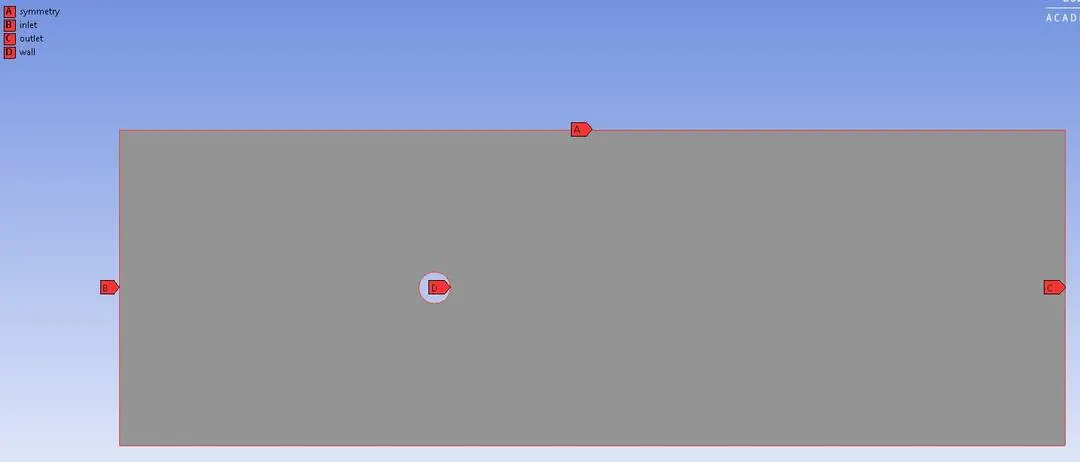
Named Selection of the created geometry.
Meshing parameters:
Mesh Type = traingular mesh.
Mesh cell size = 0.5m
No. of inflation layers = 6.
Height of the first inflation layer = 0.005m.
Divisions at the circumference of the cylinder = 36.
growth rate = 1.2
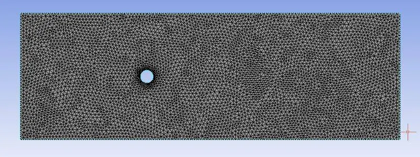
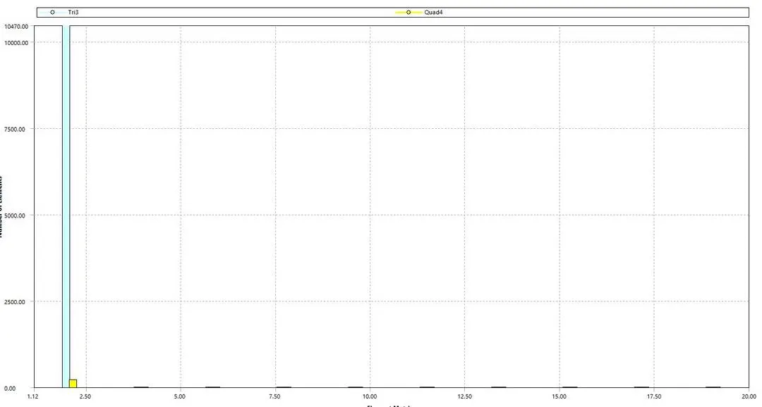
No. of Mesh elements= 10686.
Inflation layers at the circumference of the cylinder.
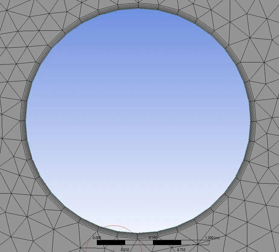
The circumference of cylinder is meshed with 36 divisions to capture the curve of the circle. Usually 1 division is assigned for every `10^o` angle on the curvature.
Mesh quality.
Setting up the physics for the flow.
Part1: -
The incompressible Navior Strokes equation is solved for Re 100 using steady and unsteady solver with pressure velocity coupling.
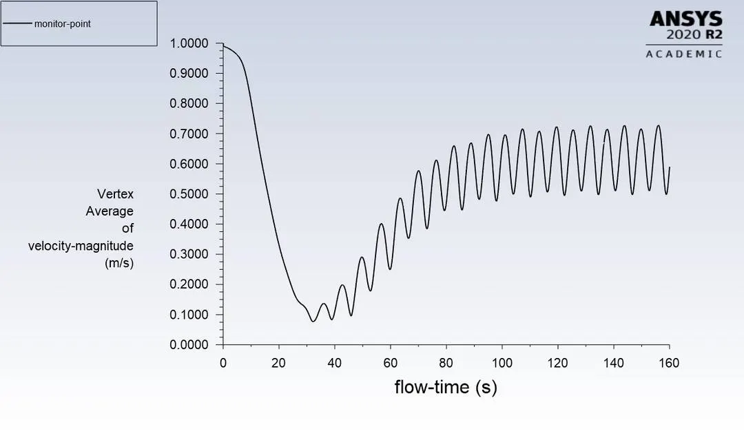
Monitor point:
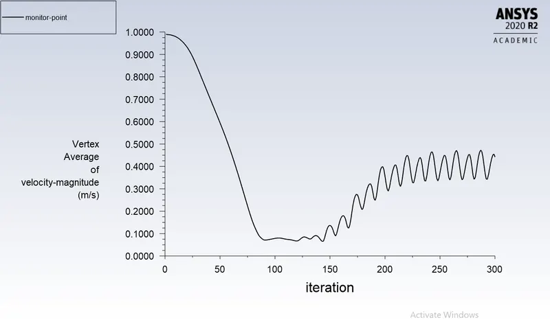
Monitor point is positioned at a distance of 4 times the diameter of the cylinder towards the outlet boundary to measure the velocity variation after the flow separation.
Material Properties:
Material = air.
Density `rho` = 1 kg/`m^3`.
Dynamic Viscosity(`mu`) = 0.02 kg/ms.
Inlet velocity v= 1m/s.
`Re = (v.D)/(mu)` = (1.2)/0.02 = 100
Boundary condition type: Velocity inlet, pressure outlet.
The outlet pressure is set to gauge pressure of 0 Pascals. The side walls of the domain are assigned symmetry boundary conditions due to which velocity normal to the symmetry plane is zero and ensure zero gradient to all variables normal to symmetry plane. The cylinder surface is assigned wall boundary conditions which is no slip wall boundary condition.
Plots obtained using steady solver.
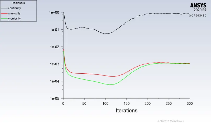
Residual Plot
Velocity at monitor point.
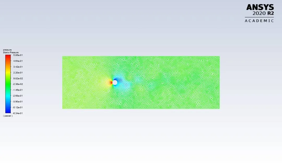
Pressure Contour.
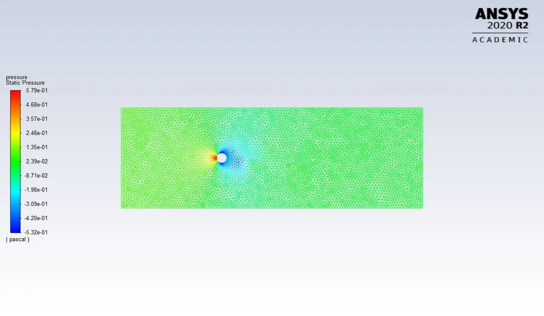
From the contour plot the stagnation point at the front of the cylinder and the flow separation happening on the surface of the cylinder can be seen
Velocity Contour
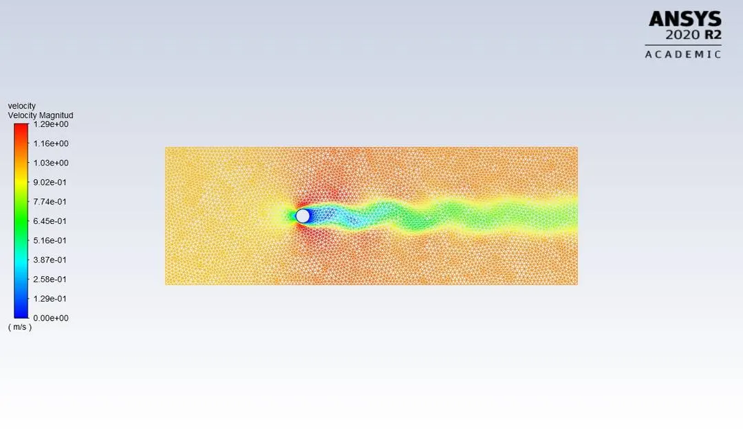
Plots obtained using Transient solver.
Residual Plot.
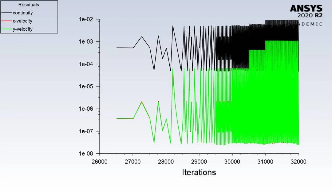
Velocity at monitor point.
Pressure Plot:
Velocity plot
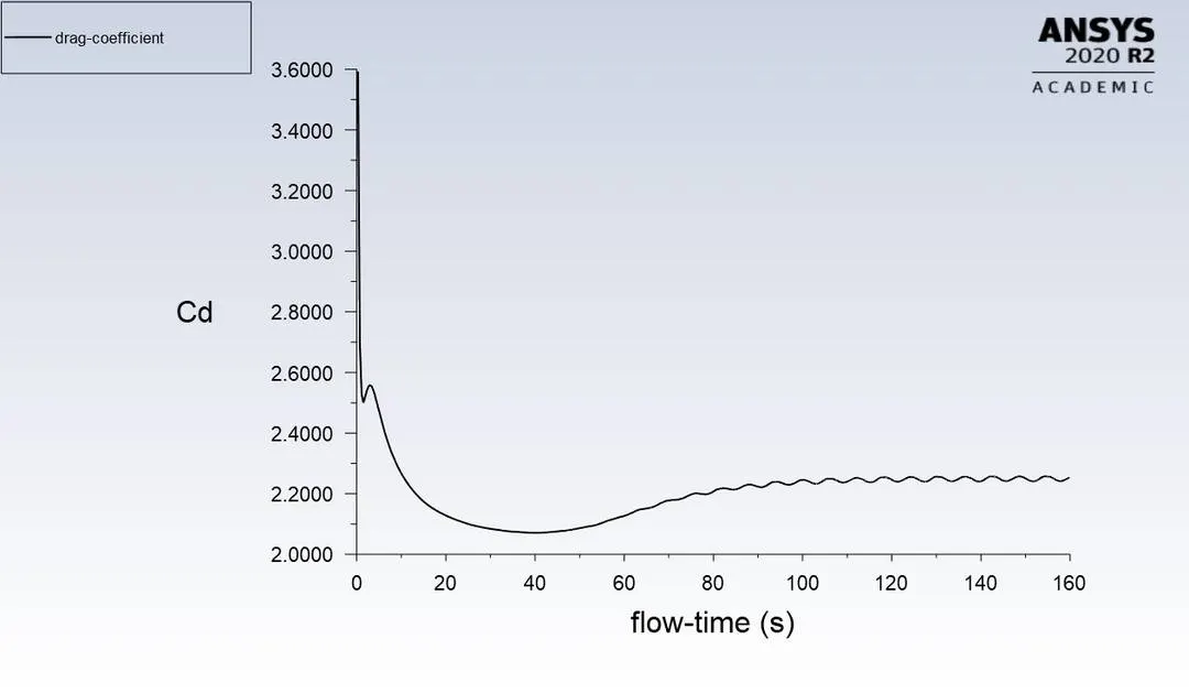
Drag Coefficient:
Lift coefficient.
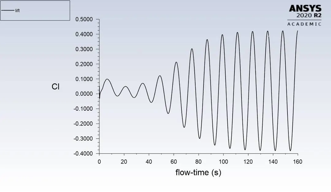
Calculation for Strouhal Number.
`St = (f.D)/v`
`f = 2.5/(30) = 0.0833` Hz.
`St = (0.83.2)/1 =0.166 `
Inference:
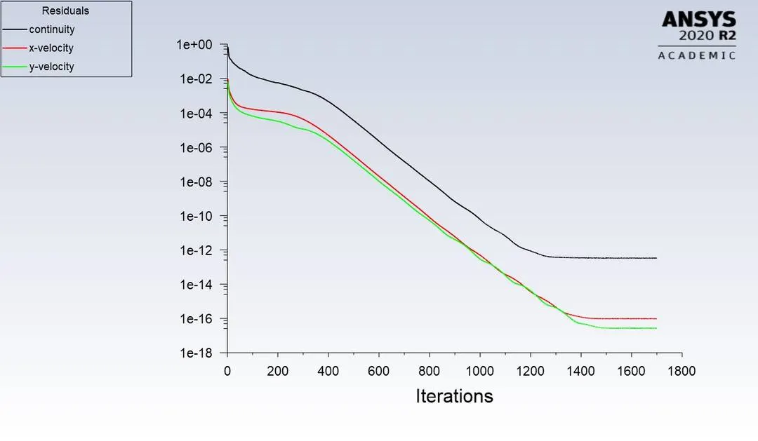
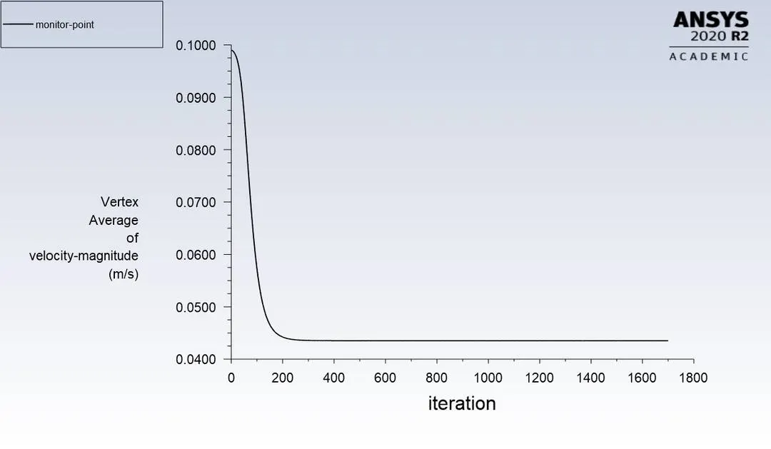
From Residual plot after 250 iterations the residuals are constant and also from velocity at monitor point follows the same pattern hence we can conclude that the solution has reached a steady state thus there will be no change in the resulting solution even if there is increase in the number of the solution.
In the simulation using steady state solver, the results are not time accurate due to which we cannot calculate the Strauhal number whereas in the simulation using unsteady solver the accurate solutions can be obtained from Strauhal number can be calculated which is 0.166.
Part II:
In this part the simulation is done for the range of Reynolds number by varying the velocity of the flow at the inlet and simulated using steady state solver.
Case 1: Re = 10.
Here Velocity v = 0.1m/s.
Residual plot:
Velocity at the monitor point
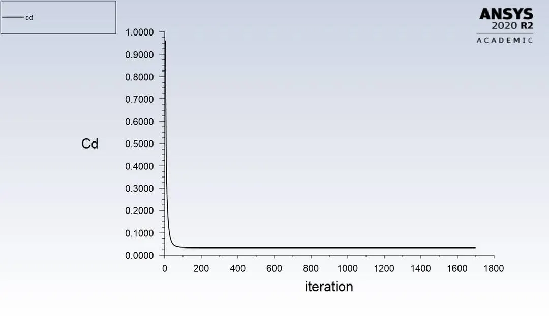
Coefficient of Drag
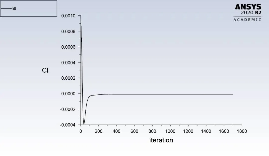
Coefficient of lift
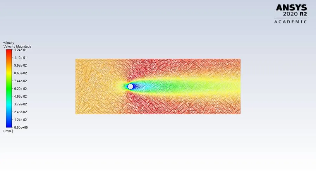
Velocity contour plot
Case 2: Re=100
Velocity v = 1m/s
Residual plot:
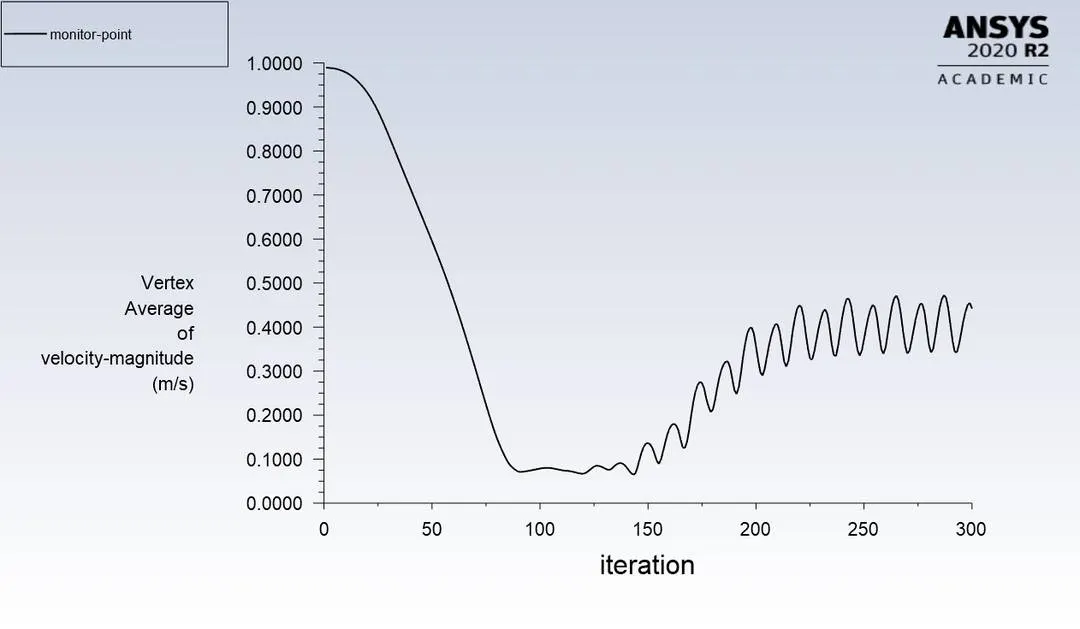
Velocity at the monitor point.
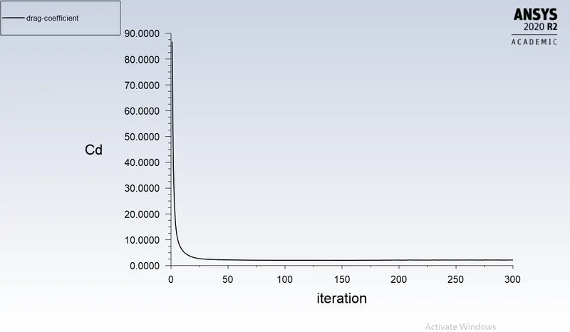
Coefficient of Drag
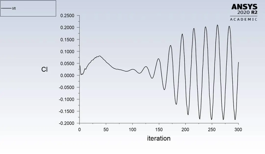
Coefficient of lift
Velocity contour plot
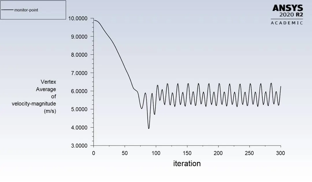
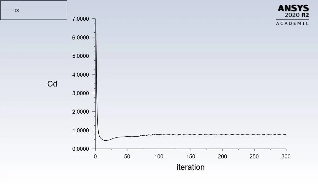
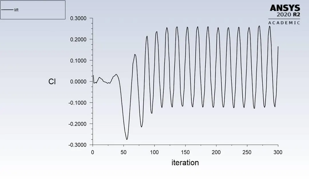
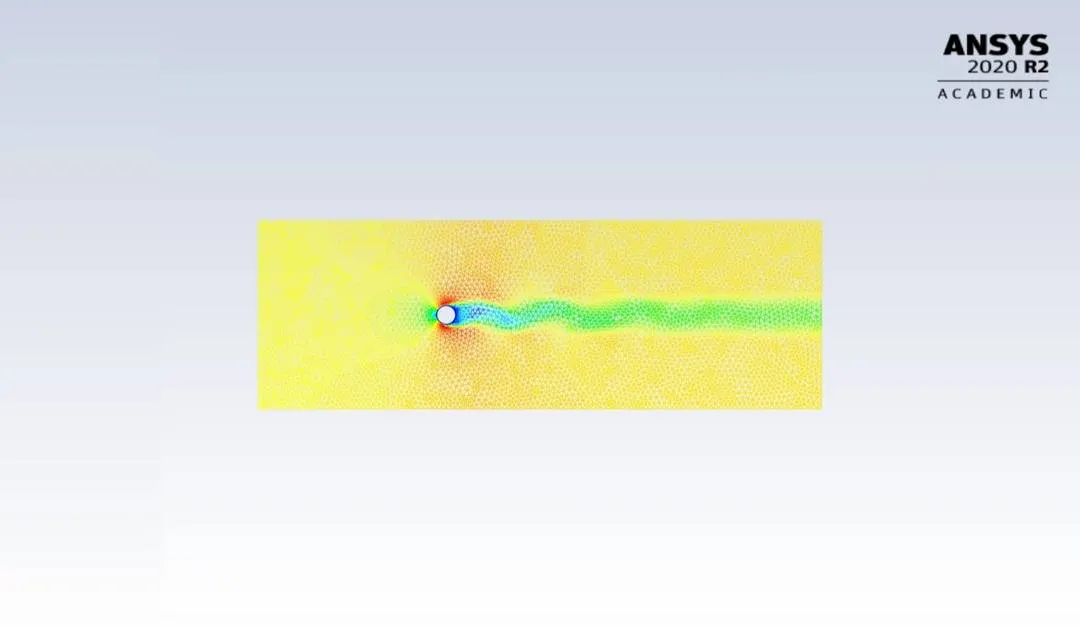
Case 3: Re=1000
Velocity v = 10m/s
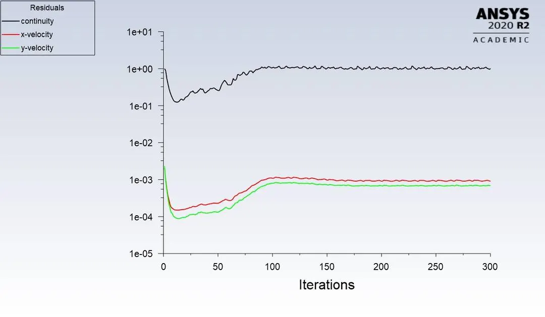
Residual plot:
Velocity at the monitor point
Coefficient of Drag
Coefficient of lift
Velocity contour plot
Case 4: Re=10000
Velocity v = 100m/s
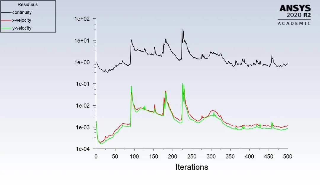
Residual plot:
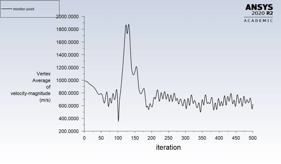
Velocity at the monitor point
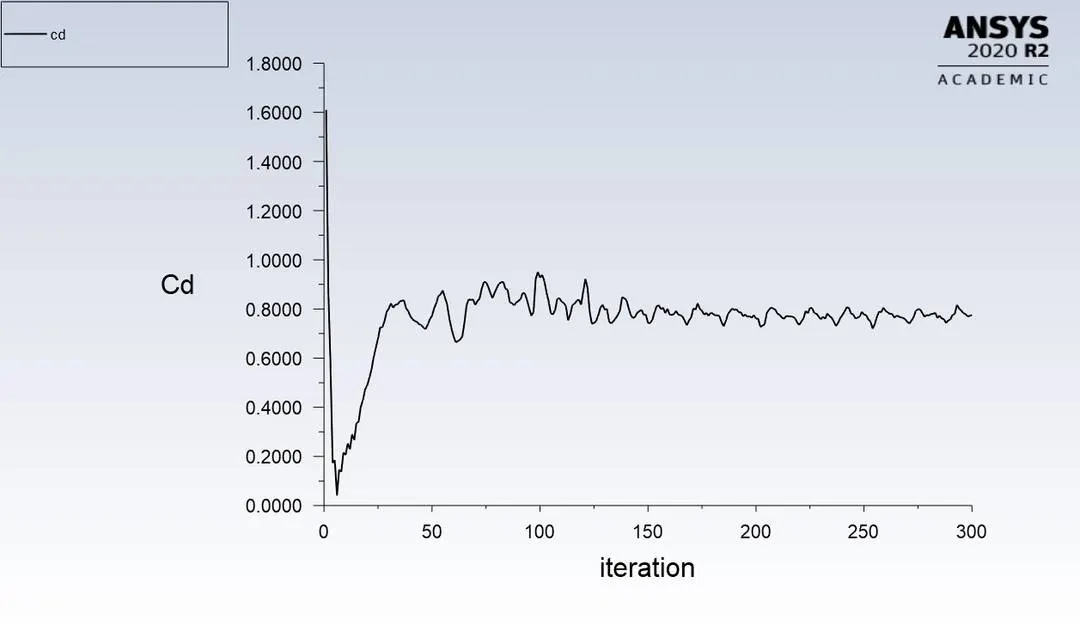
Coefficient of Drag
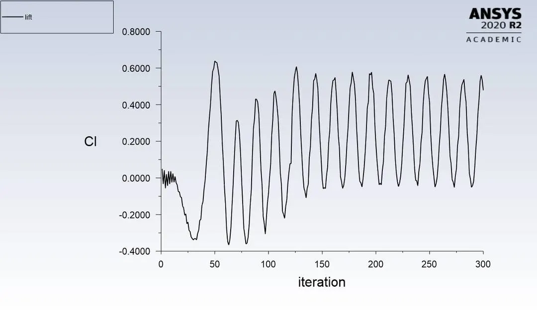
Coefficient of lift
Velocity contour plot
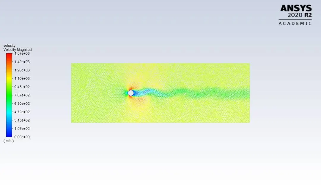
Case 5: Re=100000
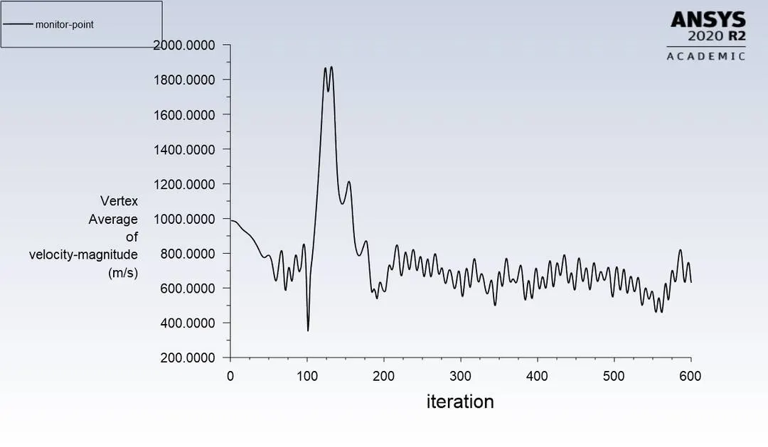
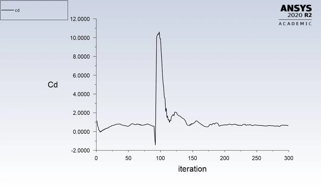
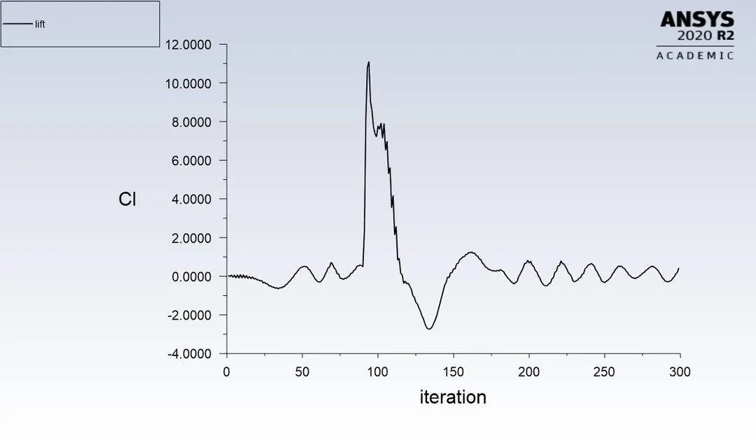
Velocity v = 1000m/s
Residual plot:
Velocity at the monitor point
Coefficient of Drag
Coefficient of lift
Velocity contour plot
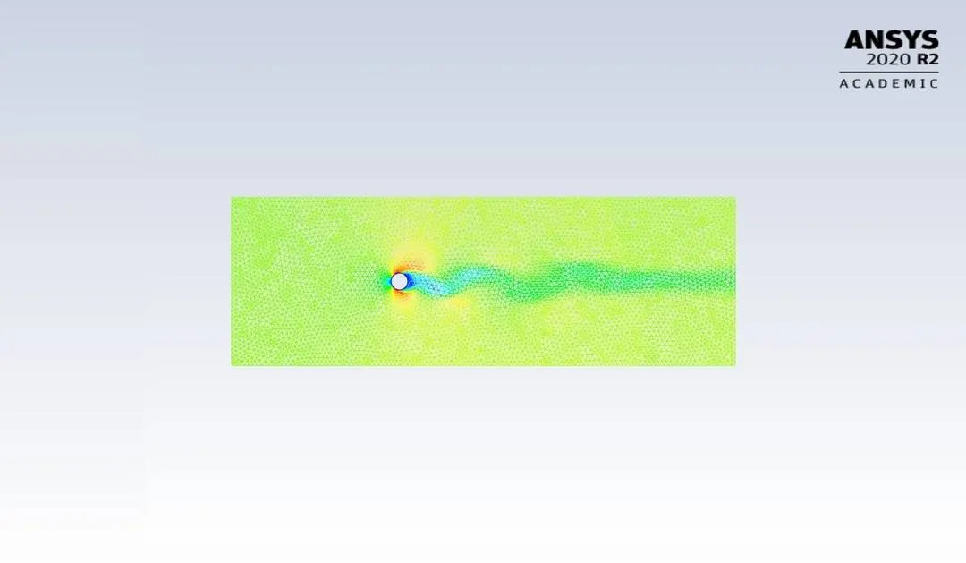
Table depicting the effect of reynolds number on drag coefficient and lift coefficient.
|
Velocity in m/s |
Reynolds Number |
Drag Coefficient |
|
0.1 |
10 |
3.3 |
|
1 |
100 |
1.32 |
|
10 |
1000 |
0.758 |
|
100 |
10000 |
0.72 |
|
1000 |
100000 |
0.62 |
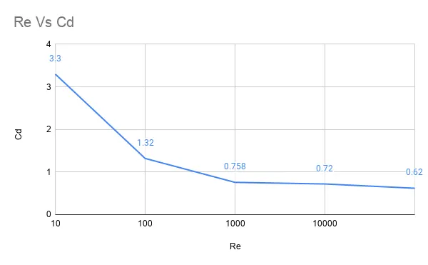
Plot Re vs Cd
Conclusion
- From the above table we can conclude that with increase in Reynolds number the coefficient of drag decreases.
- With increase in Reynolds number magnitude of the oscillation increases.
- Von Karman Vortex street is observed above a critical value of Reynolds number which is 40 which can be confirmed from the plots for Re 10 and Re 100 using steady state solver.
- There in increase in Residual values due to velocity fluctuations created because of the Karman vortex.
- The obtained results are validated with the reference material provided and found that deviation of drag coefficient for Re 10 and 100 is less than 5% and hence same procedure is followed to calculate drag coefficient for Re 1000,10000,100000. The results are plotted using values from the table.