Exhaust Port Challenge

Problem Statement:

1. Calculate the heat transfer coefficient on the internal solid surface and plot the temperature and velocity contours.

2. Explain why the Y+ is maintained within a certain range and the turbulence model chosen.

3. Verify HTC predictions from the fluent analysis and also on what factors does the accuracy of the predictions depends on.

Introduction:

Conjugate Heat Transfer Coefficient(CHT).

What is CHT?
Heat transfer is known as the flow of thermal energy from one region to another region occupied by any matter (solids and fluids) where the rate of heat transfer is proportional to the temperature difference between the regions/matter. Conjugate heat transfer (CHT) is used to describe the variation of temperature between the solids and fluids due to the exchange of thermal energy between them.

Why is CHT used in the numerical analysis?
The important parameters for any heat-transfer devices are temperature, heat flux, and heat transfer coefficient of the surfaces exposed to heating or cooling environment. However accurate calculation of convective heat transfer coefficient requires boundary conditions consist of the coupling of solid and fluid fields. Such boundary conditions assume that the heat convected in or out to or from the solid is absorbed from or rejected by the fluid passing over the solid surface. This situation is highly complex to analyze theoretically since the wall and freestream parameters vary from time to time. So, an analytical solution for the simplest case of heat transfer problem necessitates a lot of simplified assumptions. Conventionally the solution for the problem has been sought explicitly for fluid and solid. That means the heat conduction in the solid is solved by assuming a constant or time-dependent heat flux at the solid boundary and the flowfield is analyzed with the assumption of either constant wall heat flux or isothermal wall boundary. However, the isothermal wall boundary condition is far away from reality in most of the practical heat transfer situations. Hence the heat transfer coefficient prediction employing isothermal boundary layer condition is also found to be erroneous To have the analytical or numerical prediction of heat transfer coefficient close to experimentally obtained values, one must focus on conjugating the boundary condition at the fluid-solid interface through a couple of heat transfer analysis. Such a coupled field study is termed as Conjugate Heat Transfer (CHT) analysis.

Applications of CHT analysis:

Applications of the CHT is widespread. Some of them are in heat treatment of materials in the manufacturing processes. The study of heat transfer and temperature distribution of the material as it undergoes various manufacturing phases. CHT analysis not restricted to manufacturing sectors but also in gas turbine blade cooling, thermocouple design, design and sizing of heat exchangers, furnace design, aerospace applications, etc

The reason for the choice for the particular range of Y+ and turbulence model is chosen.

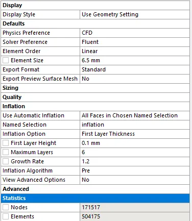
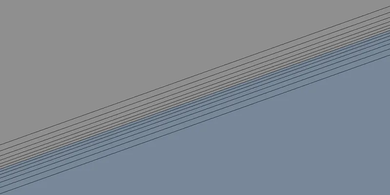
The Y+ values are maintained below 10, as the heat transfer coefficient is wall phenomenon inflation layers are created by assigning first-layer thickness of 0.1 mm to the interference layer between solid and fluid domain. By decreasing the thickness of the inflation layers Y+ values are maintained below 10. As the heat transfer coefficient is the interested parameter for this problem and it is the wall phenomenon hence K-omega turbulence model is used as it is efficient in solving boundary layer problems and also the range of Y+ values is in favor of this turbulence model.

Modeling of the geometry:

The volume is extracted for the fluid flow using the volume extract command in the prepare menu.

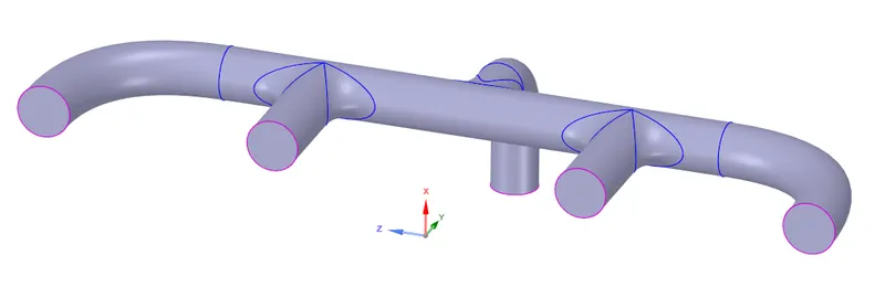
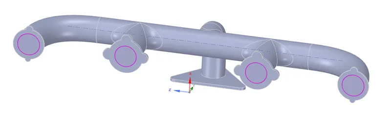
The inner volume and outer wall are combined using the share command in the workbench menu. This is done for the exchange of information between the fluid wall and solid wall and also to prevent nonconformal walls formed during mesh that is creating floating nodes.

Mesh parameters:

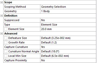
Mesh Parameters for the outer body

Meshed Model:

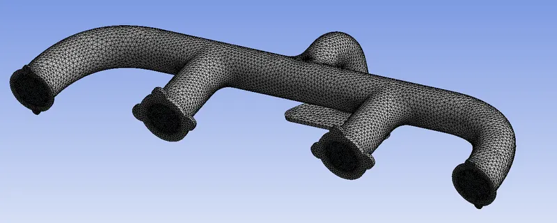
Inflation layers at the interference of solid and fluid volume.

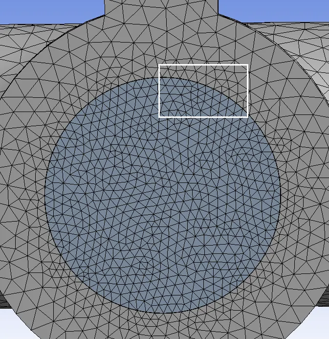
Inflation layers at the highlighted region.

Setting up physis for the given problem:

Physis:

K-omega turbulence model is chosen because of the chosen inflation layer thickness which influences the Y+ range.

Material:

Air

Density: `rho = 1.225 (kg)/m^3`

Specific Heat: `cp=1006.43 J/(Kg -K)`

Thermal Conductivity: `k=0.0242 W/(m-K)`

Dynamic Viscosity: `mu =1.7894×10^5 (kg)/(m-s)`

The solid material used for the pipe is aluminum with the material properties:

Density: `rho = 2719 (kg)/m^3`

Specific Heat: `cp=871 J/(Kg -K)`

Thermal Conductivity: `k=202.4 W/(m-K)`

Boundary condition type: Velocity inlet, pressure outlet.

The outlet pressure is set to gauge pressure of 0 Pascals. The interference wall between solid and fluid volume is given as a wall boundary condition because we are measuring the heat transfer coefficient at this layer. The outer wall is also assigned wall boundary condition with a forced convection coefficient of 20 `W/(m^2 K)` and a free stream temperature of 300K. The initialization of the solution is done using hybrid initialization.

A steady solver is used for this simulation.

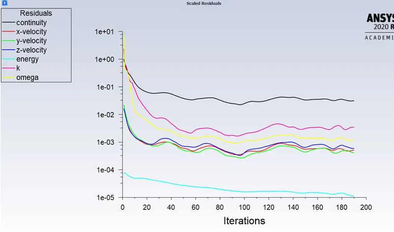
Residual Plot:

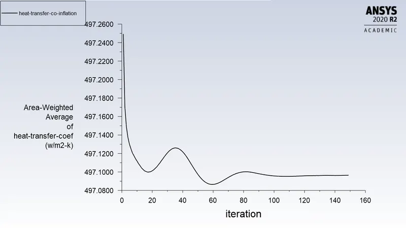
Weighted Average Heat Transfer Co-efficient:

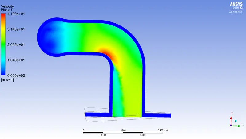
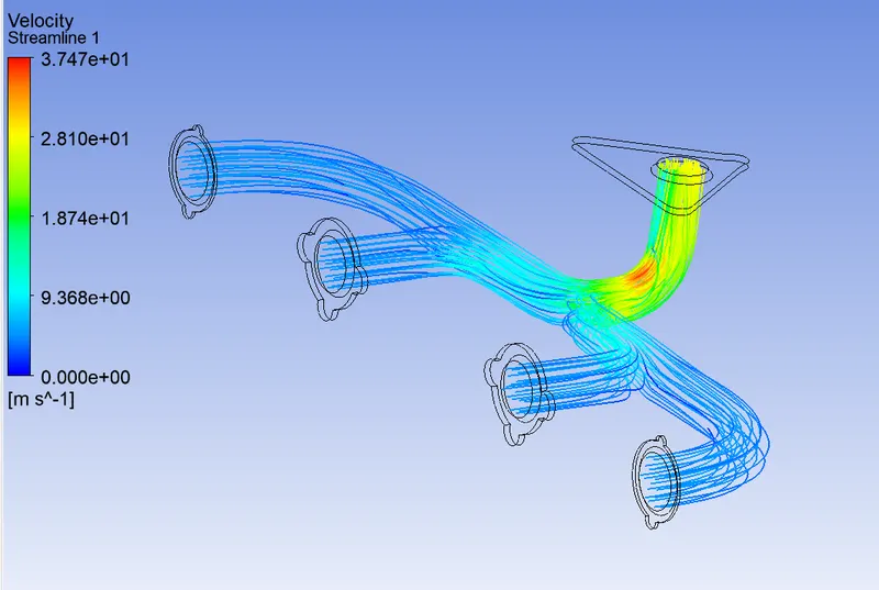
Velocity Contour Plot at the outlet.

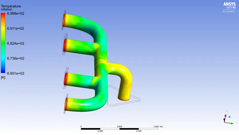
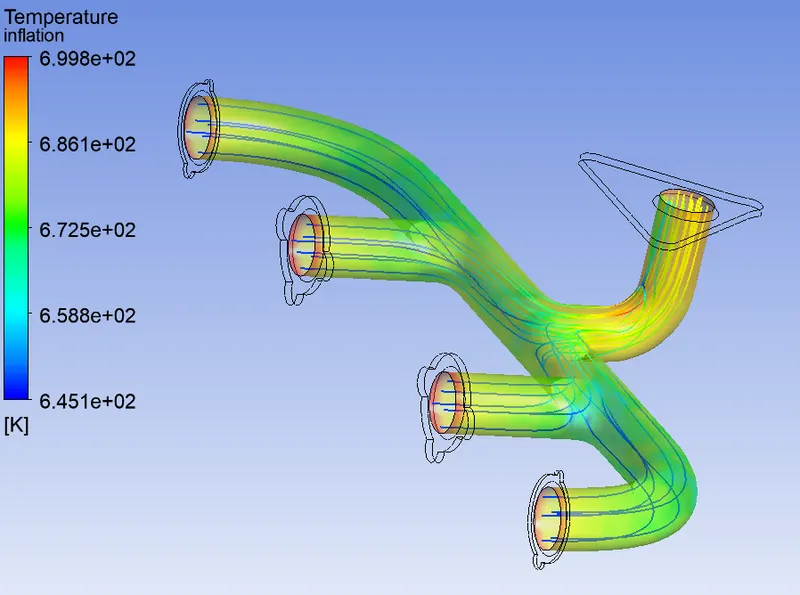
Temperature Contour Plot:

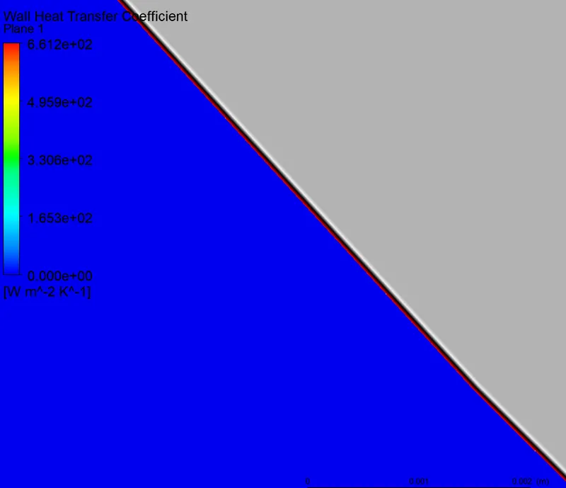
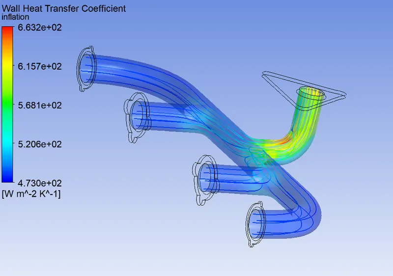
Wall heat Transfer Coefficient:

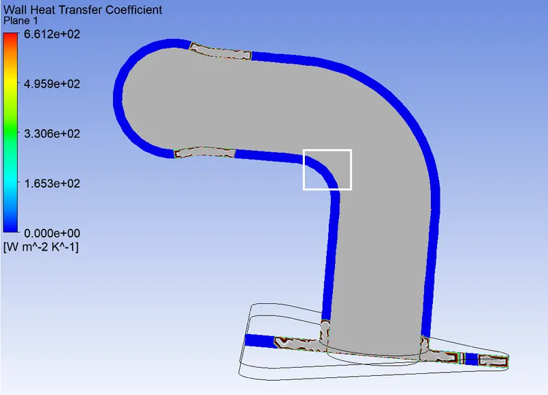
Highlighted section:

Velocity Streamlines starting from the inlet.

Plot for temperature with velocity streamlines.

Plot for Wall heat transfer co-efficient with velocity streamlines.

Grid independence Test:

Mesh Element size	No. of Elements	Wall Heat Transfer Co-efficient.
Outer wall = 50mm Inner volume = 50mm Inflation first layer thickness = 0.1 mm	209653	635.5
Outer wall = 50mm Inner volume = 5mm	360324	651.5
Outer wall = 20mm Inner volume = 6.5mm	504175	661.2

Conclusion:

From the above plots, we can infer that there is an increase in velocity at the bend near the outlet because of the flow due to mixing. Due to the increase in velocity at this point the temperature and wall heat transfer coefficient is highest. But with the coarse mesh which has relatively larger elements and no inflation layers which produced was not able to capture this effect as a result the wall heat transfer coefficient produced is lower when compared to refined mesh. The heat transfer coefficient for different mesh sizes is shown in the grid independence table.

Through experimental methods, we can determine the temperature difference and hence the heat loss/gain through the system. The Nusselt number can be calculated from this data which leads to the calculation of the heat transfer coefficient. There are various empirical relations that can help calculate the Nusselt number analytically. The widely used correlations for flow in a pipe are the Gnielinski correlation and the Dittus-Boelter equation. The Dittus-Boelter equation can be used to calculate the Nusselt number from the Reynolds' number and Prandtl number of the flow.

`Nu = 0.023.Re^0.8.Pr^(1/3)`

`h = (Nu*K)/L`

As there is no experimental analysis done previously for the given exhaust manifold design, the values obtained for the heat transfer coefficient could not be validated. We can infer from the grid dependency test that without the inflation layers the flow is not accurately simulated and hence the heat transfer coefficient is also low compared to one with the refined mesh. And at the point of maximum velocity heat transfer coefficient should be maximum which is seen from the above plots and hence we can conclude that the simulation is done is following the physics and with the refining of the mesh, the HTC value increases which conclude that the simulation is done correctly.

The factors on which the heat transfer coefficient depends are geometry, the temperature of the flowing fluid in the region, fluid to wall temperature ratio, the inlet velocity of the fluid flowing, and also thermal properties of the fluid such as Heat capacity, viscosity, etc. Hence care should be taken in specifying values to the above-mentioned parameters when solving for heat transfer coefficients.