Week 2 Air standard Cycle

Problem Statement:

1. Write a code to solve an Otto Cycle and plot a PV graph.

2. Output the thermal efficiency for the same.

Introduction:

Otto Cycle:

Otto cycle is used in internal combustion engines. It follows the 4 states that is 1->2 is isentropic compression process, 2->3 is isochoric heat addition process, 3->4 is isentropic expansion process, 4->1 is isochoric heat rejection process.

Formulas:

1.

i.`R= "connecting rod length"/"crankpin radius"`

`"Crankpin radius (a)" = "stroke length"/2`

`r_c` is compression ratio

`theta` is the crank angle.

2. `Volume swept = pi/4 * d^2. L`

where d is bore diameter in m.

L is the stroke length in m.

3.`"Clearance Volume" = "Volume swept"/(compression ratio-1)`

4.`V1 = swept volume + "clearance volume"`

5. `V2 = "Clearance volume"`

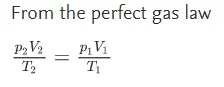
6.

7. Isentropic Compression Process

`P1V1^gamma = P2V2^gamma`

8. Thermal Efficiency

`eta = 1- Cr^(1-gamma)`

Intial Conditions

bore diameter = 0.1m

stroke length = 0.1m.

compression ratio = 12

connecting rod ratio = 1

P1 = 101325 Pascals.

T1 = 500K

Tmax = T3 = 2300K.

`gamma`= 1.4.

Logic Used:

The pressure, volume, and temperature are calculated sequentially from state 1 to state 4.

The change in volume and pressure during the isentropic compression and expansion process is calculated using the ode function.

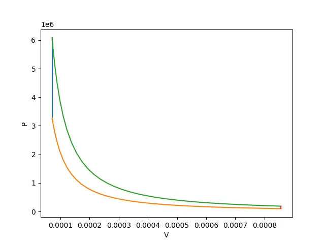
A graph is plotted for P vs V for different 4 states.

Code:

import math
import matplotlib.pyplot as plt

#inputs
#bore diameter in m
b= 0.1
#stroke length in m
stroke=0.1
#connecting rod length in m
connrod=0.15

gamma=1.4

#compression ratio
cr=12

#Function to calculate the change in volume in compression stroke and expansion stroke for corresponding change in angle.
def engine_kinematics(b,stroke,connrod,start_crank,end_crank):
	a=stroke/2
	R=connrod/a

	V_s = math.pi*(1/4)*pow(b,2)*stroke
	V_c = V_s/(cr-1)

#Starting crank angle in radians.
	sc = math.radians(start_crank)
# Ending crank angle in radians.
	ec = math.radians(end_crank)

#Noumber of values of the angle between start and end crank angle.
	n = 50
#Interval between between each angle
	dtheta=(ec-sc)/(n-1)

	V=[]

#For loop to calculate the volume for each angle.
	for i in range (0,n):
		theta = sc+i*dtheta
		term1 = 0.5*(cr-1)
		term2 = R+1-math.cos(theta)
		term3 = pow(R,2)-pow(math.sin(theta),2)
		term4 = pow(term3,0.5)

		V.append((1+term1*(term2-term4))*V_c)

	return V
	

# Swept volume
V_s = math.pi*(1/4)*pow(b,2)*stroke
#Clearance volume
V_c = V_s/(cr-1)

v1 = V_c+V_s
v2 = V_c
#Inputs

#Stage 1
p1 = 101325
t1 = 500

#State 2
p2 = p1*pow(v1,gamma)/pow(v2,gamma)
t2 =(p2*v2*t1)/(p1*v1)

#Calling the function engine_kinematics to calculate the change in volume for corresponding change in crank angle
V_compression = engine_kinematics(b,stroke,connrod,0,180)
constant = p1*pow(v1,gamma)
p_compression=[]

for v in V_compression:
	p_compression.append(constant/pow(v,gamma))


#State 3
v3=v2
#Temperature at combustion
t3 = 2500
p3 = (p2*v2*t3)/(t2*v3)

#Calling the function engine_kinematics to calculate the change in volume for corresponding change in crank angle
V_expansion = engine_kinematics(b,stroke,connrod,0,180)
constant = p3*pow(v3,gamma)

p_expansion=[]

for v in V_expansion:
	p_expansion.append(constant/pow(v,gamma))

#Stage 4
v4=v1
p4 = p3*pow(v3,gamma)/pow(v4,gamma)

#thermal efficiency
efficiency = 1-(1/pow(cr,gamma))
print(efficiency)

#Plotting of graph
plt.plot([v2,v3],[p2,p3])
plt.plot(V_compression,p_compression)
plt.plot(V_expansion,p_expansion)
plt.plot([v4,v1],[p4,p1])
plt.xlabel("V")
plt.ylabel("P")
plt.savefig("PV diagram.png")
plt.show()

Explanation.

The pressure, volume, and temperature are found sequentially from state 1- state 4.

The pressure and temperature for the isentropic compression and expansion process is found out by using

Isentropic Compression Process

`P1V1^gamma = P2V2^gamma`

Isentropic Expansion Process

`P3V3^gamma = P4V4^gamma`

The pressure and temperature for constant volume heat addition and heat rejection are found out using the perfect gas law equation.

Use of function:

The function created is used for the calculation of change in volume during the isentropic compression and expansion process.

Graph:

Inference:

From the above graph, the orange curve represents the compression stroke and the green curve represents the expansion stroke. and blue and red lines represent the constant volume compression and expansion stroke respectively.

The efficiency of the otto cycle for the given input is 0.969